
File size: 2,933 Bytes
18f5e08 | 1 2 3 4 5 6 7 8 9 10 11 12 13 14 15 16 17 18 19 20 21 22 23 24 25 26 27 28 29 30 31 32 33 34 35 36 37 38 39 40 41 42 43 44 45 46 47 48 49 50 51 52 53 54 55 56 57 58 59 60 61 62 63 64 65 66 67 68 69 70 71 72 73 74 75 76 77 78 79 80 81 82 83 | {
"nbformat": 4,
"nbformat_minor": 0,
"metadata": {
"colab": {
"provenance": []
},
"kernelspec": {
"name": "python3",
"display_name": "Python 3"
},
"language_info": {
"name": "python"
}
},
"cells": [
{
"cell_type": "code",
"execution_count": null,
"metadata": {
"id": "WMYGesN_u0od"
},
"outputs": [],
"source": [
"import numpy as np\n",
"import matplotlib.pyplot as plt\n",
"from mpl_toolkits.mplot3d import Axes3D\n",
"\n",
"# Constants and functions\n",
"r = 0.5 # Radius of the circle\n",
"x0 = np.array([1, 1]) # Initial point\n",
"\n",
"def Y(l):\n",
" return np.array([np.cos(l), np.sin(l)])\n",
"\n",
"# Curves x(s,l)\n",
"def x(s, l):\n",
" return x0 + r * np.sin(s) * Y(l)\n",
"\n",
"# Cone function\n",
"# This function correctly now calculates a point on the cone based on s, l and t.\n",
"def cone(s, l, t):\n",
" x_sl = x(s, l)\n",
" return np.array([np.cos(t) * x_sl[0], np.sin(t) * x_sl[1], t])\n",
"\n",
"# Parametric plot of the folded cone (corrected version)\n",
"fig = plt.figure()\n",
"ax = fig.add_subplot(111, projection='3d')\n",
"\n",
"# Creating the meshgrid properly using numpy\n",
"s = np.linspace(0, np.pi/2, 50) # s (parameter along the arc)\n",
"l = np.linspace(0, 2*np.pi, 50) # l (parameter around the circle)\n",
"t = np.linspace(0, 1, 50) # t (parameter along the cone height)\n",
"\n",
"# Using NumPy's broadcasting to compute the cone points - This avoids loops and is efficient.\n",
"S, T = np.meshgrid(s, t)\n",
"L = np.tile(l, (len(t), 1)).T # This creates a repeated array of l for each t value.\n",
"\n",
"# Now we evaluate the cone function on the grid points.\n",
"# We need to 'vectorize' our cone function for it to work on arrays.\n",
"cone_pts = np.vectorize(cone, signature='(),(),()->(n)')(S, L, T)\n",
"\n",
"# We extract X, Y, Z coordinates for plotting\n",
"X = cone_pts[..., 0]\n",
"Y = cone_pts[..., 1]\n",
"Z = cone_pts[..., 2]\n",
"\n",
"# Plot the surface. The surface is defined by the X, Y, Z arrays.\n",
"ax.plot_surface(X, Y, Z, alpha=0.8, cmap='viridis')\n",
"\n",
"# Combining the plot with a base circle at the bottom.\n",
"# We use the first row of X, Y since it corresponds to the base circle (t=0).\n",
"ax.plot(X[0], Y[0], np.zeros_like(X[0]), color='red', linewidth=2)\n",
"\n",
"# Hide axes for better visibility\n",
"plt.axis('off')\n",
"\n",
"# Show the plot\n",
"plt.show()"
]
}
]
} |