
Diffusers documentation
拡散モデルの学習
拡散モデルの学習
無条件画像生成は、拡散モデルの代表的な応用であり、学習に使用したデータセットの画像に似た画像を生成します。通常、特定のデータセットで事前学習済みモデルをファインチューニングすることで、最も良い結果が得られます。これらのチェックポイントはHub上で多く公開されていますが、お好みのものが見つからない場合は、ご自身でトレーニングすることもできます。
このチュートリアルでは、Smithsonian Butterflies データセットの一部を使用して、UNet2DModel をゼロから学習する方法を学び、オリジナルの🦋蝶🦋を生成します。
💡 このトレーニングチュートリアルは、Training with 🧨 Diffusersノートブックをベースにしています。拡散モデルの仕組みなど、追加の詳細や背景については、ノートブックを参照してください。
開始する前に、画像データセットの読み込みと前処理を行うための🤗 Datasets、およびGPUの台数を問わずトレーニングを簡素化するための🤗 Accelerateがインストールされていることを確認してください。以下のコマンドを実行すると、トレーニング指標を可視化するためのTensorBoardもインストールされます(トレーニングの追跡にはWeights & Biasesを使用することもできます)。
# uncomment to install the necessary libraries in Colab
#!pip install diffusers[training]
モデルをコミュニティと共有することをお勧めします。そのためには、Hugging Face アカウントへのログインが必要です(アカウントをお持ちでない場合は、こちらから作成してください)。ノートブックからログインし、プロンプトが表示された際にトークンを入力します。トークンに write ロールが付与されていることを確認してください。
>>> from huggingface_hub import notebook_login

>>> notebook_login()
または、ターミナルからログインします:
hf auth login
モデルのチェックポイントは非常に大きいため、これらの大きなファイルをバージョン管理するためにGit-LFSをインストールしてください。
!sudo apt -qq install git-lfs
!git config --global credential.helper store
トレーニング設定
利便性のため、学習ハイパーパラメータ(必要に応じて調整してください)を含むTrainingConfigクラスを作成します。
>>> from dataclasses import dataclass

>>> @dataclass
... class TrainingConfig:
...     image_size = 128  # the generated image resolution
...     train_batch_size = 16
...     eval_batch_size = 16  # how many images to sample during evaluation
...     num_epochs = 50
...     gradient_accumulation_steps = 1
...     learning_rate = 1e-4
...     lr_warmup_steps = 500
...     save_image_epochs = 10
...     save_model_epochs = 30
...     mixed_precision = "fp16"  # `no` for float32, `fp16` for automatic mixed precision
...     output_dir = "ddpm-butterflies-128"  # the model name locally and on the HF Hub

...     push_to_hub = True  # whether to upload the saved model to the HF Hub
...     hub_model_id = "<your-username>/<my-awesome-model>"  # the name of the repository to create on the HF Hub
...     hub_private_repo = None
...     overwrite_output_dir = True  # overwrite the old model when re-running the notebook
...     seed = 0


>>> config = TrainingConfig()
データセットを読み込む
🤗 Datasets ライブラリを使用して、Smithsonian Butterflies データセットを簡単に読み込むことができます:
>>> from datasets import load_dataset

>>> config.dataset_name = "huggan/smithsonian_butterflies_subset"
>>> dataset = load_dataset(config.dataset_name, split="train")
💡 HugGan Community Event で追加のデータセットを見つけることも、ローカルに
ImageFolderを作成して独自のデータセットを使用することもできます。データセットが HugGan Community Event のものである場合はconfig.dataset_nameにリポジトリ ID を、独自の画像を使用する場合はimagefolderを設定してください。
🤗 Datasets は Image 機能を使用して、画像データを自動的にデコードし、PIL.Image として読み込みます。これにより、以下のように可視化できます:
>>> import matplotlib.pyplot as plt

>>> fig, axs = plt.subplots(1, 4, figsize=(16, 4))
>>> for i, image in enumerate(dataset[:4]["image"]):
...     axs[i].imshow(image)
...     axs[i].set_axis_off()
>>> fig.show()
ただし、画像のサイズはすべて異なるため、まず前処理を行う必要があります。
Resizeは、画像のサイズをconfig.image_sizeで定義されたサイズに変更します。RandomHorizontalFlipは、画像をランダムに左右反転させることでデータセットを拡張します。Normalizeは、モデルが期待する [-1, 1] の範囲にピクセル値を再スケーリングするために重要です。
>>> from torchvision import transforms

>>> preprocess = transforms.Compose(
...     [
...         transforms.Resize((config.image_size, config.image_size)),
...         transforms.RandomHorizontalFlip(),
...         transforms.ToTensor(),
...         transforms.Normalize([0.5], [0.5]),
...     ]
... )
🤗 Datasetsのset_transformメソッドを使用して、preprocess関数をトレーニング中にオンザフライで適用します:
>>> def transform(examples):
...     images = [preprocess(image.convert("RGB")) for image in examples["image"]]
...     return {"images": images}


>>> dataset.set_transform(transform)画像を再度可視化して、リサイズが正しく行われたことを確認してみてください。これで、学習用にデータセットをDataLoaderでラップする準備が整いました!
>>> import torch

>>> train_dataloader = torch.utils.data.DataLoader(dataset, batch_size=config.train_batch_size, shuffle=True)
UNet2DModel を作成する
🧨 Diffusers の事前学習済みモデルは、望むパラメータを指定してそのモデルクラスから簡単に作成できます。例えば、UNet2DModel を作成するには:
>>> from diffusers import UNet2DModel

>>> model = UNet2DModel(
...     sample_size=config.image_size,  # the target image resolution
...     in_channels=3,  # the number of input channels, 3 for RGB images
...     out_channels=3,  # the number of output channels
...     layers_per_block=2,  # how many ResNet layers to use per UNet block
...     block_out_channels=(128, 128, 256, 256, 512, 512),  # the number of output channels for each UNet block
...     down_block_types=(
...         "DownBlock2D",  # a regular ResNet downsampling block
...         "DownBlock2D",
...         "DownBlock2D",
...         "DownBlock2D",
...         "AttnDownBlock2D",  # a ResNet downsampling block with spatial self-attention
...         "DownBlock2D",
...     ),
...     up_block_types=(
...         "UpBlock2D",  # a regular ResNet upsampling block
...         "AttnUpBlock2D",  # a ResNet upsampling block with spatial self-attention
...         "UpBlock2D",
...         "UpBlock2D",
...         "UpBlock2D",
...         "UpBlock2D",
...     ),
... )
サンプル画像の形状がモデルの出力形状と一致していることを、すばやく確認しておくのがよい場合があります。
>>> sample_image = dataset[0]["images"].unsqueeze(0)
>>> print("Input shape:", sample_image.shape)
Input shape: torch.Size([1, 3, 128, 128])

>>> print("Output shape:", model(sample_image, timestep=0).sample.shape)
Output shape: torch.Size([1, 3, 128, 128])
素晴らしい!次に、画像にノイズを追加するためにスケジューラーが必要です。
スケジューラーを作成する
スケジューラは、モデルをトレーニングに使用しているか推論に使用しているかによって、動作が異なります。推論時には、スケジューラはノイズから画像を生成します。トレーニング時には、スケジューラは拡散プロセスの特定の時点におけるモデルの出力(またはサンプル)を取得し、ノイズスケジュールと更新ルールに従って画像にノイズを適用します。
DDPMSchedulerを見てみましょう。以前使用したsample_imageにランダムなノイズを加えるために、add_noiseメソッドを使います。
>>> import torch
>>> from PIL import Image
>>> from diffusers import DDPMScheduler

>>> noise_scheduler = DDPMScheduler(num_train_timesteps=1000)
>>> noise = torch.randn(sample_image.shape)
>>> timesteps = torch.LongTensor([50])
>>> noisy_image = noise_scheduler.add_noise(sample_image, noise, timesteps)

>>> Image.fromarray(((noisy_image.permute(0, 2, 3, 1) + 1.0) * 127.5).type(torch.uint8).numpy()[0])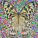
モデルの学習目的は、画像に追加されたノイズを予測することです。このステップでの損失は、次の式で計算できます。
>>> import torch.nn.functional as F

>>> noise_pred = model(noisy_image, timesteps).sample
>>> loss = F.mse_loss(noise_pred, noise)
モデルを学習
ここまでで、モデルの学習を開始するための大部分の要素が揃い、あとはそれらを組み立てるだけです。
まず、optimizerとlearning rate schedulerが必要です:
>>> from diffusers.optimization import get_cosine_schedule_with_warmup

>>> optimizer = torch.optim.AdamW(model.parameters(), lr=config.learning_rate)
>>> lr_scheduler = get_cosine_schedule_with_warmup(
...     optimizer=optimizer,
...     num_warmup_steps=config.lr_warmup_steps,
...     num_training_steps=(len(train_dataloader) * config.num_epochs),
... )次に、モデルを評価する方法が必要です。評価には、DDPMPipelineを使用してサンプル画像のバッチを生成し、グリッドとして保存できます。
>>> from diffusers import DDPMPipeline
>>> from diffusers.utils import make_image_grid
>>> import os

>>> def evaluate(config, epoch, pipeline):
...     # Sample some images from random noise (this is the backward diffusion process).
...     # The default pipeline output type is `List[PIL.Image]`
...     images = pipeline(
...         batch_size=config.eval_batch_size,
...         generator=torch.Generator(device='cpu').manual_seed(config.seed), # Use a separate torch generator to avoid rewinding the random state of the main training loop
...     ).images

...     # Make a grid out of the images
...     image_grid = make_image_grid(images, rows=4, cols=4)

...     # Save the images
...     test_dir = os.path.join(config.output_dir, "samples")
...     os.makedirs(test_dir, exist_ok=True)
...     image_grid.save(f"{test_dir}/{epoch:04d}.png")
これにより、🤗 Accelerate を使用して、TensorBoard によるログ記録、勾配の蓄積、混合精度学習を簡単に実行できるトレーニングループに、これらのコンポーネントをすべて組み込むことができます。モデルを Hub にアップロードするには、リポジトリ名と情報を取得する関数を作成し、それを Hub にプッシュします。
💡 以下の学習ループは長く、複雑に見えるかもしれませんが、後で1行のコードで学習を開始できることを考えると、その価値は十分にあります。今すぐ画像生成を始めたい場合は、以下のコードをコピーして実行してください。モデルの学習が完了するのを待っている間など、後でいつでも戻ってきて、学習ループをより詳しく確認できます。🤗
>>> from accelerate import Accelerator
>>> from huggingface_hub import create_repo, upload_folder
>>> from tqdm.auto import tqdm
>>> from pathlib import Path
>>> import os

>>> def train_loop(config, model, noise_scheduler, optimizer, train_dataloader, lr_scheduler):
...     # Initialize accelerator and tensorboard logging
...     accelerator = Accelerator(
...         mixed_precision=config.mixed_precision,
...         gradient_accumulation_steps=config.gradient_accumulation_steps,
...         log_with="tensorboard",
...         project_dir=os.path.join(config.output_dir, "logs"),
...     )
...     if accelerator.is_main_process:
...         if config.output_dir is not None:
...             os.makedirs(config.output_dir, exist_ok=True)
...         if config.push_to_hub:
...             repo_id = create_repo(
...                 repo_id=config.hub_model_id or Path(config.output_dir).name, exist_ok=True
...             ).repo_id
...         accelerator.init_trackers("train_example")

...     # Prepare everything
...     # There is no specific order to remember, you just need to unpack the
...     # objects in the same order you gave them to the prepare method.
...     model, optimizer, train_dataloader, lr_scheduler = accelerator.prepare(
...         model, optimizer, train_dataloader, lr_scheduler
...     )

...     global_step = 0

...     # Now you train the model
...     for epoch in range(config.num_epochs):
...         progress_bar = tqdm(total=len(train_dataloader), disable=not accelerator.is_local_main_process)
...         progress_bar.set_description(f"Epoch {epoch}")

...         for step, batch in enumerate(train_dataloader):
...             clean_images = batch["images"]
...             # Sample noise to add to the images
...             noise = torch.randn(clean_images.shape, device=clean_images.device)
...             bs = clean_images.shape[0]

...             # Sample a random timestep for each image
...             timesteps = torch.randint(
...                 0, noise_scheduler.config.num_train_timesteps, (bs,), device=clean_images.device,
...                 dtype=torch.int64
...             )

...             # Add noise to the clean images according to the noise magnitude at each timestep
...             # (this is the forward diffusion process)
...             noisy_images = noise_scheduler.add_noise(clean_images, noise, timesteps)

...             with accelerator.accumulate(model):
...                 # Predict the noise residual
...                 noise_pred = model(noisy_images, timesteps, return_dict=False)[0]
...                 loss = F.mse_loss(noise_pred, noise)
...                 accelerator.backward(loss)

...                 if accelerator.sync_gradients:
...                     accelerator.clip_grad_norm_(model.parameters(), 1.0)
...                 optimizer.step()
...                 lr_scheduler.step()
...                 optimizer.zero_grad()

...             progress_bar.update(1)
...             logs = {"loss": loss.detach().item(), "lr": lr_scheduler.get_last_lr()[0], "step": global_step}
...             progress_bar.set_postfix(**logs)
...             accelerator.log(logs, step=global_step)
...             global_step += 1

...         # After each epoch you optionally sample some demo images with evaluate() and save the model
...         if accelerator.is_main_process:
...             pipeline = DDPMPipeline(unet=accelerator.unwrap_model(model), scheduler=noise_scheduler)

...             if (epoch + 1) % config.save_image_epochs == 0 or epoch == config.num_epochs - 1:
...                 evaluate(config, epoch, pipeline)

...             if (epoch + 1) % config.save_model_epochs == 0 or epoch == config.num_epochs - 1:
...                 if config.push_to_hub:
...                     upload_folder(
...                         repo_id=repo_id,
...                         folder_path=config.output_dir,
...                         commit_message=f"Epoch {epoch}",
...                         ignore_patterns=["step_*", "epoch_*"],
...                     )
...                 else:
...                     pipeline.save_pretrained(config.output_dir)
ふー、かなり多くのコードになりましたね!ついに🤗 Accelerateのnotebook_launcher関数を使ってトレーニングを開始する準備が整いました。トレーニングループ、すべてのトレーニング引数、そしてトレーニングに使用するプロセス数(この値は利用可能なGPUの数に変更できます)を関数に渡します:
>>> from accelerate import notebook_launcher

>>> args = (config, model, noise_scheduler, optimizer, train_dataloader, lr_scheduler)

>>> notebook_launcher(train_loop, args, num_processes=1)
トレーニングが完了したら、拡散モデルによって生成された最終的な🦋画像🦋を確認してください!
>>> import glob

>>> sample_images = sorted(glob.glob(f"{config.output_dir}/samples/*.png"))
>>> Image.open(sample_images[-1])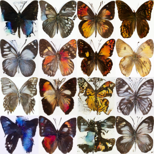
次のステップ
無条件画像生成は、学習可能なタスクの一例です。🧨 Diffusers Training Examplesページにアクセスして、他のタスクや学習手法を探索できます。以下は、学習できる内容の例です。
- Textual Inversionは、モデルに特定の視覚的概念を学習させ、生成された画像にそれを統合するアルゴリズムです。
- DreamBoothは、対象の複数の入力画像から、その対象のパーソナライズされた画像を生成する技術です。
- ガイド:独自のデータセットで Stable Diffusion モデルをファインチューニングする方法。
- ガイド: LoRAは、非常に大規模なモデルをより高速にファインチューニングするためのメモリ効率の高い手法です。