Tempo-GENCO: Learning the Grid Solver of Tomorrow

Carlo Siebenschuh, Brian Hsu: University of Chicago, Argonne National Laboratory:
siebenschuh@uchicago.edu

Static AC optimal power flow (AC-OPF) surrogates predict optimal operating states, while grid operators must anticipate uncertain future conditions. We introduce Tempo-GENCO, a 91k-parameter temporal adapter that extends a frozen 20M-parameter foundation model to probabilistic day-ahead forecasting from 72 hours of operating history. Training combines the energy score with a power-balance penalty. Experiments span grids with up to 2,000 buses on Aurora and NVIDIA systems. Detailed evaluation on four grids, using three training seeds, 72 test origins, and 64 trajectories per forecast, shows improved joint energy scores over climatology and a forecast-then-solve baseline. Overconfidence and increased physical residuals remain challenges. These results demonstrate that lightweight temporal adaptation can extend a static optimization surrogate without jointly training both components from scratch. Code is available on GitHub and as the Python package power-fm-foresight.

1. Introduction

Snapshot-based AC optimal power flow (AC-OPF) datasets cast neural optimization surrogates as graph-to-vector regression: given a network and its loads, predict the optimal operating state. But grid operators don't work from snapshots. They have to anticipate how demand will evolve and how contingencies will play out, with effects that ripple across both time and the network. We ask whether a geometric foundation model trained only on static grids can pick up this temporal capability through a lightweight adapter—one that consumes a history of operating states and jointly forecasts future conditions together with their AC-optimal states. Forecasts of this kind could help operators plan dispatch and reserves ahead of time, and flag congestion as it begins to emerge.

Since future conditions are uncertain, the target is really a distribution over optimal operating trajectories. For such forecasts to be useful, they need to express that uncertainty honestly while staying physically plausible, so we train with a proper scoring rule and evaluate calibration alongside forecast accuracy and constraint violations. Beyond the forecasting task itself, this probes how far GENCO's learned representations actually reach: whether the physical and operational structure it absorbed from static graphs gives it a useful foundation for temporal adaptation, even though the backbone was never trained to model dynamics.

2. Method

Predict the optimum, not its inputs.
A grid operator never sees demand alone but a sequence of operating points. At hour $t$ the realised demand $d_t$ fixes the optimal state through the AC optimal power flow (AC-OPF) map

$$x_t^{\ast }=S(d_t):=\arg \underset{x\in \mathcal{X}}{\min }c(x)\text{s.t.}F(x,d_t)=0,x\_t^\{\backslash ast\}\; \backslash ;=\backslash ;\; S(d\_t)\; \backslash ;:=\backslash ;\; \backslash arg\backslash min\_\{x\backslash in\backslash mathcal\; X\}\backslash ;\; c(x)\; \backslash quad\backslash text\{s.t.\}\backslash quad\; F(x,\; d\_t)\; =\; 0,$$

where $F$ collects the AC power-balance equations, $\mathcal X$ the box and thermal limits, and $x=(|V|,\theta,P_g,Q_g)$. The day-ahead object of interest is the conditional law of tomorrow's trajectory $X_t^{\ast}=(x^{\ast}{t+1},\dots,x^{\ast}{t+24})$ given the history $H_t$ of the last $72$ solved hours and the calendar $c$. The classical pipeline forecasts the inputs and solves afterwards, i.e. it targets the push-forward $S_{#},\mathbb P(d_{t+1:t+24}\mid H_t,c)$ one scenario at a time; every scenario costs a nonconvex solve, forecast error is amplified through $S$ in a way the forecaster never sees, and the two stages are tuned to different objectives. We instead learn the push-forward end to end and sample the future optimum directly,

$${\mathrm{T}\mathrm{e}\mathrm{m}\mathrm{p}\mathrm{o}}_{\theta }\circ \mathrm{G}\mathrm{E}\mathrm{N}\mathrm{C}\mathrm{O}:(H_t,c)⟼{\widehat{\mathbb{P}}}_{\theta }\text{\hspace{0.17em}⁣}\left(X_t^{\ast }\right|H_t,c)\approx \{{\widehat{X}}_1,\dots ,{\widehat{X}}_K\},\backslash mathrm\{Tempo\}\_\{\backslash theta\}\backslash circ\backslash mathrm\{GENCO\}\backslash ;:\backslash ;(H\_t,\; c)\backslash ;\backslash longmapsto\backslash ;\; \backslash widehat\{\backslash mathbb\; P\}\_\{\backslash theta\}\backslash !\backslash left(X\_t^\{\backslash ast\}\backslash ,\backslash middle|\backslash ,H\_t,\; c\backslash right)\; \backslash ;\backslash approx\backslash ;\backslash \{\backslash hat\; X\_1,\backslash dots,\backslash hat\; X\_K\backslash \},$$

so that the forecast uncertainty is already expressed in the coordinates an operator acts on (dispatch, voltages, branch loadings) rather than in a demand vector that still has to be pushed through a solver.

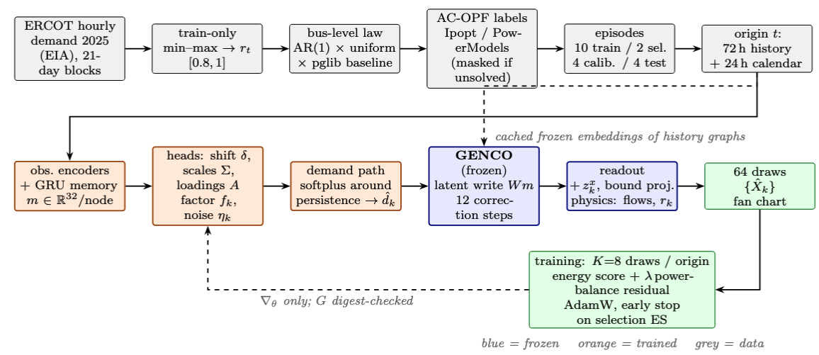
Tempo-GENCO workflow. Top: ERCOT-driven data generation, AC-OPF labels, and forecast origins. Bottom: adapter sampling (orange) through frozen GENCO (blue), with $K$ draws scored by the energy score and a residual penalty during training.

Sampler and objective.
GENCO is the backbone model, a geometric surrogate $G$ of the AC-OPF map above that maps a demand graph to an approximate optimum in twelve correction steps. A $91$k-parameter adapter $\mathrm{Tempo}_\theta$ steers it: a recurrent encoder compresses $H_t$ into a per-node memory $m=\mathrm{Enc}_\theta(H_t)$, and one draw $k$ is

$$z_k=A_{\theta }(m,c)f_k+{\mathrm{\Sigma }}_{\theta }(m,c){\eta }_k,{\widehat{d}}_k={\sigma }_{+}\text{\hspace{0.17em}⁣}({\sigma }_{+}^{-1}(d_{t-1})+{\delta }_{\theta }(m,c)+z_k^d),{\widehat{x}}_k=G({\widehat{d}}_k;W_{\theta }m,z_k^x),z\_k\; =\; A\_\backslash theta(m,c)\backslash ,f\_k\; +\; \backslash Sigma\_\backslash theta(m,c)\backslash ,\backslash eta\_k,\backslash qquad\; \backslash hat\; d\_k\; =\; \backslash sigma\_+\backslash !\backslash big(\backslash sigma\_+^\{-1\}(d\_\{t-1\})\; +\; \backslash delta\_\backslash theta(m,c)\; +\; z\_k^\{d\}\backslash big),\backslash qquad\; \backslash hat\; x\_k\; =\; G\backslash big(\backslash hat\; d\_k;\backslash ;\; W\_\backslash theta\; m,\backslash ;\; z\_k^\{x\}\backslash big),$$

with $f_k\sim\mathcal N(0,I_8)$ a factor shared by all buses and lead hours, $\eta_k\sim\mathcal N(0,I)$ diagonal noise, and $\sigma_+$ the softplus keeping demand positive around persistence. The memory enters $G$ as a write $W_\theta m$ into its input latent, and the innovations $z_k^{x}$ are added to its final readout; the backbone's own physics layers then return branch flows and the power-balance residual $r_k$ of each draw. The adapter is trained on $K$ draws per origin with the fair energy score and a residual penalty,

$$\mathcal{L}(\theta )=\underset{{\mathrm{E}\mathrm{S}}_K(\text{strictly proper})}{\underbrace{\frac{1}{K}\sum _k\mathrm{\parallel }{\widehat{X}}_k-X_t^{\ast }\mathrm{\parallel }-\frac{1}{2K(K-1)}\sum _{k\mathrm{\ne }l}\mathrm{\parallel }{\widehat{X}}_k-{\widehat{X}}_l\mathrm{\parallel }}}+\lambda \frac{1}{K}\sum _k\mathrm{\parallel }{r}_k{\mathrm{\parallel }}^2,\backslash mathcal\; L(\backslash theta)\backslash ;=\backslash ;\; \backslash underbrace\{\backslash frac1K\backslash sum\_\{k\}\backslash |\backslash hat\; X\_k\; -\; X\_t^\{\backslash ast\}\backslash |\; -\; \backslash frac\{1\}\{2K(K-1)\}\backslash sum\_\{k\backslash neq\; l\}\backslash |\backslash hat\; X\_k-\backslash hat\; X\_l\backslash |\}\_\{\backslash mathrm\{ES\}\_K\backslash ;(\backslash text\{strictly\; proper\})\}\; \backslash ;+\backslash ;\backslash lambda\backslash ,\backslash frac1K\backslash sum\_k\; \backslash |r\_k\backslash |^2\; ,$$

in train-scaled coordinates, with $G$ frozen throughout. The energy score is a strictly proper scoring rule: its expectation is minimised only by the true conditional law, so it rewards calibration and sharpness jointly and penalises both

3. Results

3.1 Tempo-GENCO as a day-ahead forecaster

TL;DR: GENCO, a geometric foundation model for AC-OPF, can be turned into a day-ahead probabilistic forecaster through a thin temporal adapter.
We refer to the model as Tempo-GENCO. The adapter reads a history of solved network states, summarizes them via a recurrent unit, and writes that memory into GENCO's input latent before its twelve correction steps.
Tempo-GENCO then produces tomorrow's optimal dispatch and operating state. No external demand forecast is supplied. Tempo-GENCO samples its own future demand implicitly to build the future graph, but — as the controls show — the source of the forecasting capability comes from steering the frozen solver's latent state. A 91k-parameter write into the input latent is enough to re-aim a 20M-parameter physics solver at tomorrow's operating point.

Details: The adapter reads 72 hours of solved network states, to predict tomorrow's optimal power flow. We measure probabilistic forecast skill via the energy score (lower is better); calibration is assessed separately through interval coverage. The GENCO backbone is chosen according to the grid size. The temporal adapter is 91k parameters in size and is trained for at most six hours on a single accelerator tile while the backbone stays frozen.
Three baselines isolate the mechanism: First, climatology of solved training days usually offers a calibrated prediction but tends to lack sharpness to be operationally useful. Second, a classical pipeline of a ridge demand forecaster with block-bootstrapped uncertainty, pushed through a frozen GENCO. This pipeline separates temporal prediction (ridge) and neural surrogate optimization (GENCO). Third, a demand control where Tempo-GENCO is used to sample demand that is pushed through unconditioned GENCO. This isolates the source of the advantage: If the adapter's advantage were a better demand forecast, it would match it. In contrast, if it comes from latent conditioning, demand control should resemble the outcome of classical pipeline; as both lack conditioning. All modes share origins, targets, coordinate scales and the scorer.

Empirics: We ran experiments on four grids (14, 30, 57, 118 buses), three training seeds, 72 test origins and $K=64$ trajectories per forecast. Tempo-GENCO has the best joint energy score everywhere: 0.70–0.90 of climatology and from 0.93 down to 0.25 of the classical pipeline as the grid grows. The demand control is never better than the classical pipeline. These results are robust as spreads between seeds (2e-3 to 3e-2) are about an order of magnitude below the gaps. The advantage is largest on generator dispatch, where Tempo-GENCO beats climatology at every lead hour on every grid, and smallest on voltage, where it is about 2-3$\times$ sharper than climatology. However, it loses to it on case118 at every lead.

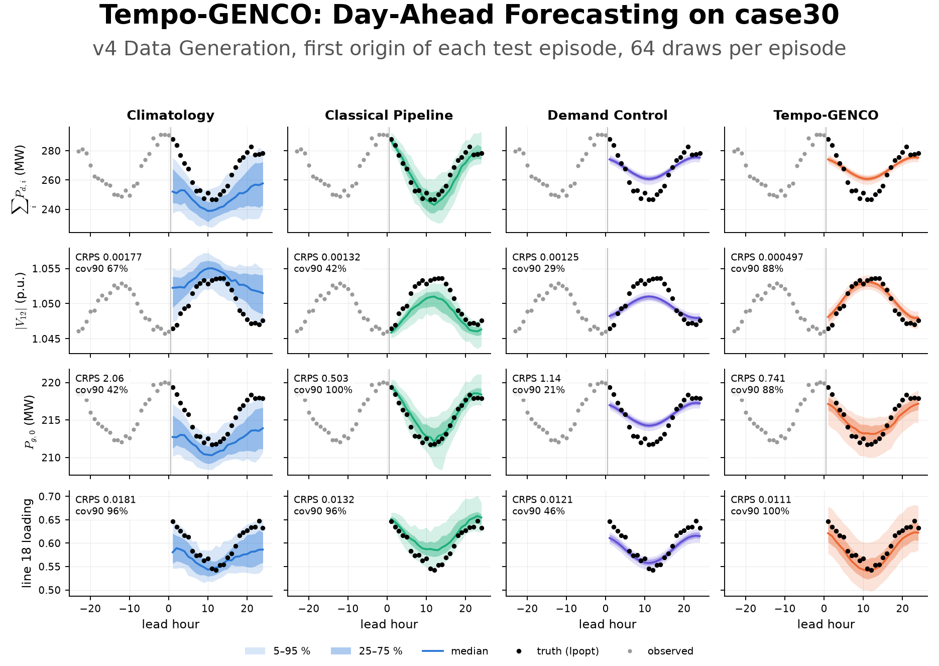
Figure 1. CAPTION 1

Table 1. Day-ahead forecast skill on the v4 data generation. Joint ES uses train-derived coordinate scales and is comparable only within a grid; ES / C is the ratio to climatology. $\lvert V_i \rvert$ columns are over all buses: fair CRPS (Continuously Ranked Probability Score, ↓), empirical coverage of the nominal 90 % band, and mean band width (sharpness). Free $P_g$ MAE is the ensemble-mean error (↓) over the free generators. $\lvert \Delta P_i \rvert$ is the mean absolute nodal active-power residual of the raw samples. Tempo-GENCO and Demand Control on case14, case57 and case118 are means over three training seeds; case30 is the run shown in Figure 1. Bold marks the best value per column (closest to 90 % for coverage).

Discussion: These experiments indicate that GENCO's latent space can be conditioned for temporal data, even though no temporal indexing entered its pre-training corpus. In fact, linear probes for next state's prediction were not successful. Hence, the latent space is a control surface the temporal adapter leverages, not a representation of dynamics. Temporal adaption comes at a cost. First, in terms of physics: prediction accuracy may conflict with physical viability. Tempo-GENCO's power-balance residual is 13-30$\times$ that of the frozen solver's as a result of the forecasting requirement. The appendix A0 ablation (conditioning removed) and the $\lambda$ sweep trace the frontier between forecast skill and physical consistency. Second, calibration. Nominal 90% voltage intervals cover only 7–41$%$. While small ensembles (with three members) recover $46%$ on case30, at an improved skill, forecasts remain overconfident. Finally, the performance ceiling induced by the backbone. GENCO's approximation error grows with grid size by an order of magnitude (the error in $|V_{i}|$ grows from 5e-4 to 4.9e-3 p.u.) and on case118 exceeds climatology's entire voltage forecast error. Naturally, the adapter inherits this floor from its frozen backbone. The same mechanism, around 50$\times$ larger outside the pretraining load range (v3 data regime), explains why the adapter's relative gain is largest there.

Further experiments: Forecasting systems find strength in the number of models involved. We assemble deep ensembles and assess if they improve forecasting accuracy and physical viability. Moreover, we analyze how robust Tempo-GENCO is when temporal dynamics deviate.

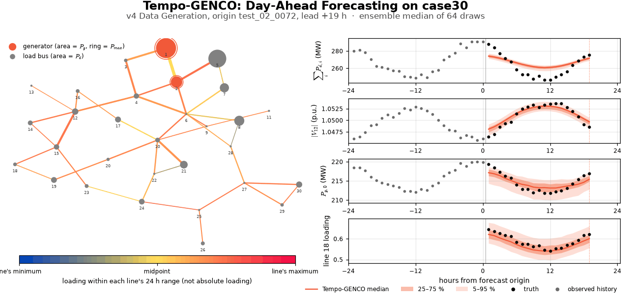
Figure 2. CAPTION 2

Discussion

Our evaluation spans Aurora and NVIDIA systems but remains non-exhaustive. We focus on GENCO, one of several AC-OPF foundation models; GridSFM and LUMINA could, in principle, support analogous temporal adaptation.

Zero-shot transfer to unseen temporal regimes remains challenging, and forecasts remain overconfident despite explicitly modeling uncertainty—a familiar calibration problem in neural networks. Nevertheless, Tempo-GENCO demonstrates that temporal forecasting and neural optimization need not be learned jointly from scratch: a lightweight adapter can extend a frozen static surrogate to probabilistic prediction of future operating states.

Related Work

@article{puech2025gridfmdatakitv1pythonlibraryscalable,
  title={gridfm-datakit-v1: A Python Library for Scalable and Realistic Power Flow and Optimal Power Flow Data Generation},
  author={Alban Puech and Matteo Mazzonelli and Celia Cintas and Tamara R. Govindasamy and Mangaliso Mngomezulu and Jonas Weiss and Matteo Baù and Anna Varbella and François Mirallès and Kibaek Kim and Le Xie and Hendrik F. Hamann and Etienne Vos and Thomas Brunschwiler},
  journal={arXiv preprint arXiv:2512.14658},
  year={2025},
  url={https://arxiv.org/abs/2512.14658}
}

@article{puech2026gencounifiedneural,
  title={GENCO - A Unified Neural Solver Embedded in a Development Framework for Steady-State Grid Analysis},
  author={Alban Puech and Matteo Mazzonelli and Tamara R. Govindasamy and Mangaliso Mngomezulu and Héctor Maeso-García and Thomas Tolhurst and Javad Bayazi and Ali Moeini and Naomi Simumba and Celia Cintas and David Nelischer and Romeo Kienzler and Jonas Weiss and Anna Varbella and Florian Dörfler and Gabriela Hug and Martin Mevissen and Juan Bernabé-Moreno and François Mirallès and Hendrik F. Hamann and Etienne Vos and Thomas Brunschwiler},
  journal={arXiv preprint arXiv:2608.09921},
  year={2026},
  url={https://arxiv.org/abs/2608.09921}
}

@article{wachter2006implementation,
  title={On the implementation of an interior-point filter line-search algorithm for large-scale nonlinear programming},
  author={W{\"a}chter, Andreas and Biegler, Lorenz T},
  journal={Mathematical programming},
  volume={106},
  number={1},
  pages={25--57},
  year={2006},
  publisher={Springer}
}

@inproceedings{coffrin2018powermodels,
  title={Powermodels. jl: An open-source framework for exploring power flow formulations},
  author={Coffrin, Carleton and Bent, Russell and Sundar, Kaarthik and Ng, Yeesian and Lubin, Miles},
  booktitle={2018 Power Systems Computation Conference (PSCC)},
  pages={1--8},
  year={2018},
  organization={IEEE}
}

@misc{eia_erco,
  author = {{U.S. Energy Information Administration}},
  title  = {Hourly Electric Grid Monitor: Electric Reliability Council of Texas ({ERCO})},
  url    = {https://www.eia.gov/electricity/gridmonitor/dashboard/electric_overview/balancing_authority/ERCO},
  note   = {Accessed: 2026-10-24}
}