
Diffusers documentation
Marigold 컴퓨터 비전
Marigold 컴퓨터 비전
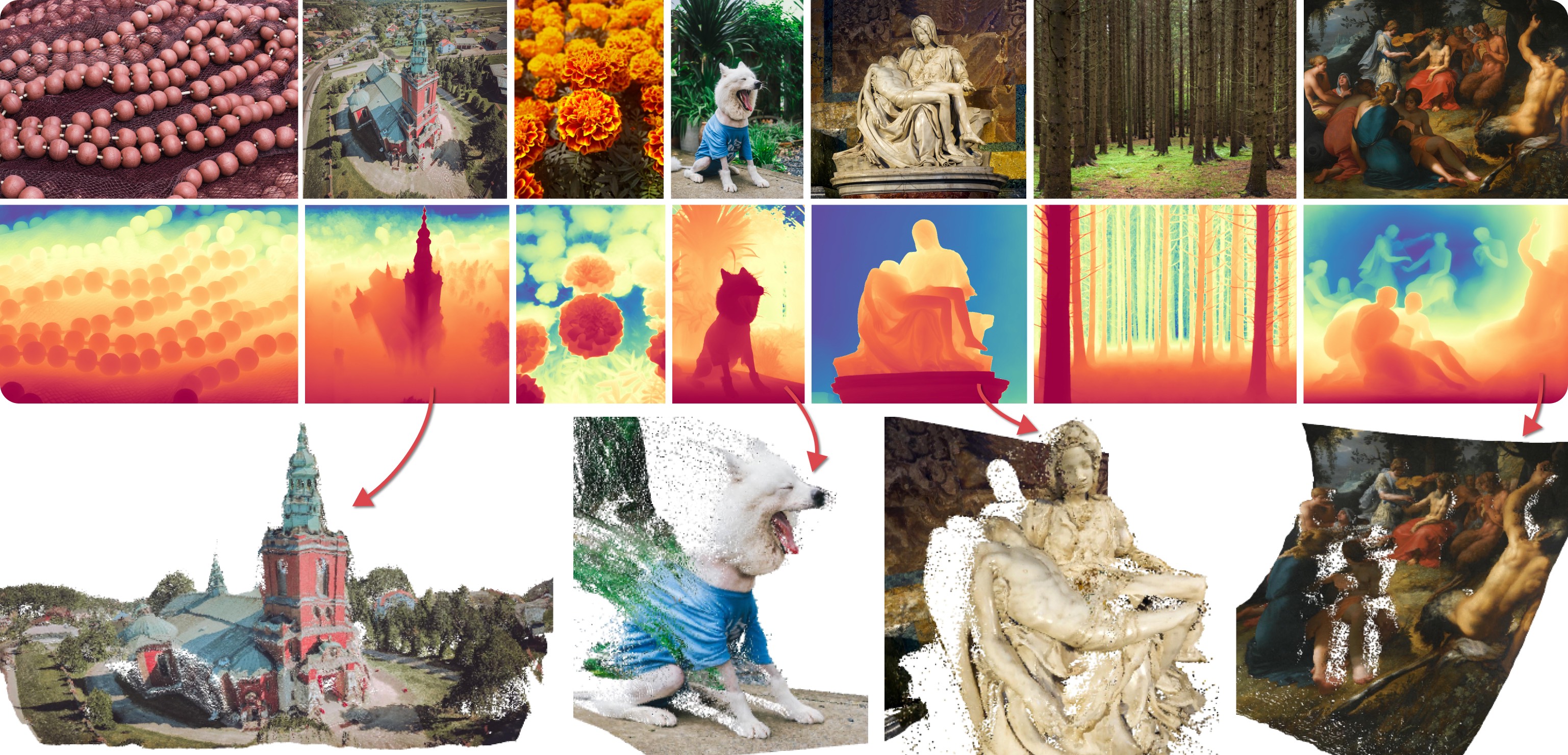
Marigold은 Bingxin Ke, Anton Obukhov, Shengyu Huang, Nando Metzger, Rodrigo Caye Daudt, Konrad Schindler가 발표한 CVPR 2024 Oral 논문인 Repurposing Diffusion-Based Image Generators for Monocular Depth Estimation에서 제안되었습니다. 핵심 아이디어는 Text-to-Image Latent Diffusion Models(LDMs)의 생성적 선験을 전통적인 컴퓨터 비전 작업에 재사용하는 것입니다. 이 접근법은 위의 티저에서 보여준 것처럼 Stable Diffusion을 Monocular Depth Estimation을 위해 파인튜닝함으로써 탐구되었습니다.
Marigold는 후속 논문 Marigold: Affordable Adaptation of Diffusion-Based Image Generators for Image Analysis에서 확장되었으며, 이 논문의 저자는 Bingxin Ke, Kevin Qu, Tianfu Wang, Nando Metzger, Shengyu Huang, Bo Li, Anton Obukhov, Konrad Schindler입니다. 이 연구는 Surface Normals와 Intrinsic Image Decomposition(IID)과 같은 새로운 모달리티를 지원하도록 Marigold를 확장하고, Latent Consistency Models(LCM)을 위한 학습 프로토콜을 도입했으며, High-Resolution(HR) 처리 기능을 입증했습니다.
초기 Marigold 모델(
v1-0및 이전 버전)은 최소 10개의 추론 단계에서 최적의 결과를 얻도록 최적화되었습니다. LCM 모델은 이후 1~4단계의 짧은 추론 단계에서도 고품질 추론을 가능하게 하도록 개발되었습니다.v1-1및 이후의 Marigold 모델은 DDIM 스케줄러를 사용하여 1~4단계의 최소 단계에서도 최적의 결과를 달성합니다.
사용 가능한 파이프라인
각 파이프라인은 특정 컴퓨터 비전 작업에 맞게 설계되어 입력 RGB 이미지를 처리하고 이에 해당하는 예측을 생성합니다. 현재 구현된 컴퓨터 비전 작업은 다음과 같습니다:
사용 가능한 체크포인트
모든 원래 체크포인트는 Hugging Face의 PRS-ETH 조직에서 사용할 수 있습니다. 이들은 diffusers 파이프라인 및 original codebase와 함께 사용하도록 설계되었으며, 새로운 모델 체크포인트를 학습하는 데에도 사용할 수 있습니다. 다음은 권장 체크포인트의 요약으로, 모두 1~4단계로 신뢰할 수 있는 결과를 생성합니다.
| 체크포인트 | 모달리티 | 댓글 |
|---|---|---|
| prs-eth/marigold-depth-v1-1 | 깊이 | Affine-invariant depth prediction은 각 픽셀에 0(근접 평면)에서 1(원거리 평면) 사이의 값을 할당하며, 두 평면 모두 추론 과정에서 모델에 의해 결정됩니다. |
| prs-eth/marigold-normals-v0-1 | Normals | 표면 법선 예측값은 화면 공간 카메라에서 -1에서 1 범위의 값을 가지는 단위 길이 3D 벡터입니다. |
| prs-eth/marigold-iid-appearance-v1-1 | Intrinsics | InteriorVerse 분해는 Albedo와 두 가지 BRDF 재료 특성인 Roughness와 Metallicity로 구성됩니다. |
| prs-eth/marigold-iid-lighting-v1-1 | Intrinsics | 이미지의 HyperSim 분해 는 Albedo $A$, Diffuse shading $S$, Non-diffuse residual $R$으로 구성됩니다: $I = A*S+R$. |
Scheduler 가이드를 확인하여 스케줄러의 속도와 품질 사이의 트레이드오프를 탐색하는 방법을 배우고, 파이프라인 간 구성 요소 재사용 섹션을 확인하여 동일한 구성 요소를 여러 파이프라인에 효율적으로 로드하는 방법을 배워보세요. 또한, 이 파이프라인의 메모리 사용량을 줄이는 방법에 대해 자세히 알고 싶다면 여기의 [“메모리 사용량 줄이기”] 섹션을 참고하세요.
Marigold 파이프라인은 모델 체크포인트에 스케줄러가 내장된 상태로 설계 및 테스트되었습니다. 최적의 추론 단계 수는 스케줄러에 따라 달라지며, 모든 경우에 가장 잘 작동하는 보편적인 값은 없습니다. 이를 위해 파이프라인의
__call__메서드에서num_inference_steps파라미터의 기본값은None입니다( API 참조를 참조하세요). 명시적으로 설정하지 않는 한, 체크포인트 구성 파일(model_index.json)의default_denoising_steps필드에서 값을 상속합니다. 이를 통해image인자만 사용하여 파이프라인을 호출할 때도 고품질의 예측을 보장합니다.
아래 예제는 대부분 깊이 예측을 위해 제시되었지만, 지원되는 다른 모달리티에도 보편적으로 적용할 수 있습니다. Midjourney로 생성된 알베르트 아인슈타인의 동일한 입력 이미지를 사용하여 예측 결과를 보여줍니다. 이를 통해 다양한 모달리티와 체크포인트 간 예측 시각화를 비교하기가 더 쉬워집니다.
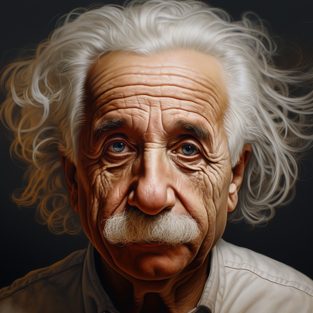
깊이 예측
깊이 예측을 얻으려면 prs-eth/marigold-depth-v1-1 체크포인트를 MarigoldDepthPipeline에 로드하고, 이미지를 파이프라인에 통과시킨 후 예측 결과를 저장합니다:
import diffusers
import torch

pipe = diffusers.MarigoldDepthPipeline.from_pretrained(
    "prs-eth/marigold-depth-v1-1", variant="fp16", dtype=torch.float16
).to("cuda")  # or "mps", "xpu", "cpu"

image = diffusers.utils.load_image("https://marigoldmonodepth.github.io/images/einstein.jpg")

depth = pipe(image)

vis = pipe.image_processor.visualize_depth(depth.prediction)
vis[0].save("einstein_depth.png")

depth_16bit = pipe.image_processor.export_depth_to_16bit_png(depth.prediction)
depth_16bit[0].save("einstein_depth_16bit.png")
visualize_depth() 함수는 matplotlib의 컬러맵(기본값은 Spectral)을 적용하여 단일 채널 [0, 1] 깊이 범위의 예측 픽셀 값을 RGB 이미지로 매핑합니다.
Spectral 컬러맵을 사용하면 가까운 깊이의 픽셀은 빨간색으로, 먼 픽셀은 파란색으로 표시됩니다.
16비트 PNG 파일은 [0, 1] 범위를 [0, 65535] 범위로 선형 매핑한 단일 채널 값을 저장합니다.
아래는 원시 예측값과 시각화된 예측값입니다. 어둡고 가까운 영역(수염)은 시각화에서 더 쉽게 구별할 수 있습니다.


표면 법선 추정
prs-eth/marigold-normals-v1-1 체크포인트를 MarigoldNormalsPipeline에 로드하고, 이미지를 파이프라인에 통과시킨 후 예측 결과를 저장합니다:
import diffusers
import torch

pipe = diffusers.MarigoldNormalsPipeline.from_pretrained(
    "prs-eth/marigold-normals-v1-1", variant="fp16", dtype=torch.float16
).to("cuda")  # or "mps", "xpu", "cpu"

image = diffusers.utils.load_image("https://marigoldmonodepth.github.io/images/einstein.jpg")

normals = pipe(image)

vis = pipe.image_processor.visualize_normals(normals.prediction)
vis[0].save("einstein_normals.png")visualize_normals()은 픽셀 값이 [-1, 1] 범위를 가지는 3차원 예측을 RGB 이미지로 매핑합니다. 시각화 함수는 좌표계의 다른 선택과 시각화가 호환되도록 표면 법선 축을 반전하는 것을 지원합니다. 개념적으로, 각 픽셀은 X 축이 오른쪽을, Y 축이 위를, Z 축이 관찰자를 향하는 좌표계에서 표면 법선 벡터에 따라 채색됩니다. 아래는 시각화된 예측입니다:

이 예시에서 코 끝은 표면의 점이 거의 확실하게 존재하며, 표면 법선 벡터가 관찰자를 정면으로 향합니다. 즉, 좌표가 [0, 0, 1]입니다.
이 벡터는 RGB [128, 128, 255]로 매핑되며, 이는 보라-파랑색에 해당합니다.
마찬가지로, 이미지 오른쪽 부분의 볼에 있는 표면 법선은 X 성분이 크며, 이는 빨간색 색조를 증가시킵니다.
위로 향하는 어깨의 점들은 Y 성분이 커서 초록색을 촉진합니다.
고유 이미지 분해
Marigold은 Intrinsic Image Decomposition(IID)을 위한 두 가지 모델, “Appearance”과 “Lighting”을 제공합니다. 각 모델은 각각 InteriorVerse와 Hypersim 어노테이션에서 파생된 Albedo 맵을 생성합니다.
- “Appearance” 모델은 또한 Roughness와 Metallicity와 같은 Material 속성을 추정합니다.
- “Lighting” 모델은 Diffuse Shading과 Non-diffuse Residual을 생성합니다.
다음은 “Appearance” 모델이 생성한 예측을 저장하는 샘플 코드입니다:
import diffusers
import torch

pipe = diffusers.MarigoldIntrinsicsPipeline.from_pretrained(
    "prs-eth/marigold-iid-appearance-v1-1", variant="fp16", dtype=torch.float16
).to("cuda")  # or "mps", "xpu", "cpu"

image = diffusers.utils.load_image("https://marigoldmonodepth.github.io/images/einstein.jpg")

intrinsics = pipe(image)

vis = pipe.image_processor.visualize_intrinsics(intrinsics.prediction, pipe.target_properties)
vis[0]["albedo"].save("einstein_albedo.png")
vis[0]["roughness"].save("einstein_roughness.png")
vis[0]["metallicity"].save("einstein_metallicity.png")
“Lighting” 모델이 생성한 예측을 보여주는 또 다른 예시입니다:
import diffusers
import torch

pipe = diffusers.MarigoldIntrinsicsPipeline.from_pretrained(
    "prs-eth/marigold-iid-lighting-v1-1", variant="fp16", dtype=torch.float16
).to("cuda")  # or "mps", "xpu", "cpu"

image = diffusers.utils.load_image("https://marigoldmonodepth.github.io/images/einstein.jpg")

intrinsics = pipe(image)

vis = pipe.image_processor.visualize_intrinsics(intrinsics.prediction, pipe.target_properties)
vis[0]["albedo"].save("einstein_albedo.png")
vis[0]["shading"].save("einstein_shading.png")
vis[0]["residual"].save("einstein_residual.png")
두 모델은 동일한 파이프라인을 공유하되 서로 다른 분해 유형을 지원합니다.
정확한 분해 매개변수화(예: sRGB 대 선형 공간)는 pipe.target_properties 사전에 저장되며, 이 사전은 visualize_intrinsics() 함수로 전달됩니다.
아래는 예측된 분해 출력을 보여주는 몇 가지 예시입니다. 모든 모달리티는 Intrinsic Image Decomposition Space에서 확인할 수 있습니다.


추론 속도 향상
위의 빠른 시작 스니펫은 이미 품질과 속도를 위해 최적화되어 있으며, 체크포인트를 로드하고 가중치 및 계산의 fp16 변형을 활용하며, 기본 수(4)의 디노이징 디퓨전 스텝을 수행합니다.
예측 품질을 희생하면서 추론을 가속화하는 첫 번째 단계는 디노이징 디퓨전 스텝을 최소로 줄이는 것입니다:
  import diffusers
  import torch

  pipe = diffusers.MarigoldDepthPipeline.from_pretrained(
      "prs-eth/marigold-depth-v1-1", variant="fp16", dtype=torch.float16
  ).to("cuda")  # or "mps", "xpu", "cpu"

  image = diffusers.utils.load_image("https://marigoldmonodepth.github.io/images/einstein.jpg")

- depth = pipe(image)
+ depth = pipe(image, num_inference_steps=1)
이 변경 사항으로 pipe 호출이 RTX 3090 GPU에서 280ms에 완료됩니다.
내부적으로 입력 이미지는 먼저 Stable Diffusion VAE 인코더를 사용하여 인코딩된 후, U-Net이 단일 디노이징
단계를 수행합니다.
마지막으로, 예측된 잠재 변수가 VAE 디코더를 통해 픽셀 공간으로 디코딩됩니다.
이 구성에서 세 가지 모듈 호출 중 두 가지는 LDM의 픽셀 공간과 잠재 공간 간의 변환에 할당됩니다.
Marigold의 잠재 공간이 Stable Diffusion 2.0과 호환되므로, 경량화된 SD VAE 대체품을 사용하면 추론 속도를 3배 이상
향상시켜 RTX 3090에서 호출 시간을 85ms로 줄일 수 있습니다.
경량화된 VAE를 사용하면 예측의 시각적 품질이 약간 저하될 수 있습니다.
  import diffusers
  import torch

  pipe = diffusers.MarigoldDepthPipeline.from_pretrained(
      "prs-eth/marigold-depth-v1-1", variant="fp16", dtype=torch.float16
  ).to("cuda")  # or "mps", "xpu", "cpu"

+ pipe.vae = diffusers.AutoencoderTiny.from_pretrained(
+     "madebyollin/taesd", dtype=torch.float16
+ ).cuda()

  image = diffusers.utils.load_image("https://marigoldmonodepth.github.io/images/einstein.jpg")

  depth = pipe(image, num_inference_steps=1)
지금까지 diffusion 단계 수와 모델 구성 요소를 최적화했습니다. Self-attention 연산은 전체 계산의 상당 부분을 차지합니다. 더 효율적인 attention processor를 사용하면 이를 가속화할 수 있습니다:
  import diffusers
  import torch
+ from diffusers.models.attention_processor import AttnProcessor2_0

  pipe = diffusers.MarigoldDepthPipeline.from_pretrained(
      "prs-eth/marigold-depth-v1-1", variant="fp16", dtype=torch.float16
  ).to("cuda")  # or "mps", "xpu", "cpu"

+ pipe.vae.set_attn_processor(AttnProcessor2_0())
+ pipe.unet.set_attn_processor(AttnProcessor2_0())

  image = diffusers.utils.load_image("https://marigoldmonodepth.github.io/images/einstein.jpg")

  depth = pipe(image, num_inference_steps=1)
마지막으로, Optimizations에서 제안한 대로 torch.compile을 활성화하면 대상 하드웨어에 따라 성능을 한층 더 향상시킬 수 있습니다.
그러나 컴파일링은 첫 번째 파이프라인 호출 시 상당한 오버헤드를 발생시키므로, 루프 내에서와 같이 동일한 파이프라인 인스턴스가 반복적으로 호출될 때만 이점이 있습니다.
  import diffusers
  import torch
  from diffusers.models.attention_processor import AttnProcessor2_0

  pipe = diffusers.MarigoldDepthPipeline.from_pretrained(
      "prs-eth/marigold-depth-v1-1", variant="fp16", dtype=torch.float16
  ).to("cuda")  # or "mps", "xpu", "cpu"

  pipe.vae.set_attn_processor(AttnProcessor2_0())
  pipe.unet.set_attn_processor(AttnProcessor2_0())

+ pipe.vae = torch.compile(pipe.vae, mode="reduce-overhead", fullgraph=True)
+ pipe.unet = torch.compile(pipe.unet, mode="reduce-overhead", fullgraph=True)

  image = diffusers.utils.load_image("https://marigoldmonodepth.github.io/images/einstein.jpg")

  depth = pipe(image, num_inference_steps=1)
정밀도 극대화 및 앙상블
Marigold 파이프라인에는 서로 다른 랜덤 라텐트에서 생성된 여러 예측을 결합하는 내장 앙상블 메커니즘이 있습니다.
이는 확산 모델의 생성적 특성을 활용하여 예측의 정밀도를 높이는 무차별적(brute-force) 방법입니다.
ensemble_size 인수가 3 이상으로 설정되면 앙상블 경로가 자동으로 활성화됩니다.
최대 정밀도를 목표로 할 경우, num_inference_steps를 ensemble_size와 동시에 조정하는 것이 적절합니다.
권장 값은 체크포인트마다 다르지만 주로 스케줄러 유형에 따라 달라집니다.
앙상블의 효과는 표면 법선(surface normals)에서 특히 잘 드러납니다:
  import diffusers

  pipe = diffusers.MarigoldNormalsPipeline.from_pretrained("prs-eth/marigold-normals-v1-1").to("cuda")  # or "mps", "xpu", "cpu"

  image = diffusers.utils.load_image("https://marigoldmonodepth.github.io/images/einstein.jpg")

- depth = pipe(image)
+ depth = pipe(image, num_inference_steps=10, ensemble_size=5)

  vis = pipe.image_processor.visualize_normals(depth.prediction)
vis[0].save("einstein_normals.png") 
…에서 볼 수 있듯이, 머리카락과 같은 세밀한 구조를 가진 모든 영역에서 예측이 더 보수적이고 평균적으로 더 정확해졌습니다. 이러한 결과는 3D 재구성처럼 정밀도에 민감한 다운스트림 작업에 더 적합합니다.
시간적 일관성을 갖춘 프레임별 비디오 처리
Marigold의 생성적 특성으로 인해 각 예측은 고유하며, 잠재 초기화에 샘플링된 무작위 노이즈에 의해 정의됩니다. 다음 비디오에서 볼 수 있듯이, 이는 전통적인 엔드투엔드 밀집 회귀 네트워크와 비교했을 때 명백한 단점이 됩니다:


이 문제를 해결하기 위해, diffusion의 시작점을 정의하는 latents 인수를 파이프라인에 전달할 수 있습니다.
경험적으로, 동일한 시작점 노이즈 latent와 이전 프레임 예측에 해당하는 latent의 볼록 조합(convex combination)이 충분히 매끄러운 결과를 제공한다는 것을 확인했으며, 아래 스니펫에 구현되어 있습니다:
import imageio
import diffusers
import torch
from diffusers.models.attention_processor import AttnProcessor2_0
from PIL import Image
from tqdm import tqdm

device = "cuda"  # or "mps", "xpu", "cpu"
path_in = "https://huggingface.co/spaces/prs-eth/marigold-lcm/resolve/c7adb5427947d2680944f898cd91d386bf0d4924/files/video/obama.mp4"
path_out = "obama_depth.gif"

pipe = diffusers.MarigoldDepthPipeline.from_pretrained(
    "prs-eth/marigold-depth-v1-1", variant="fp16", dtype=torch.float16
).to(device)
pipe.vae = diffusers.AutoencoderTiny.from_pretrained(
    "madebyollin/taesd", dtype=torch.float16
).to(device)
pipe.unet.set_attn_processor(AttnProcessor2_0())
pipe.vae = torch.compile(pipe.vae, mode="reduce-overhead", fullgraph=True)
pipe.unet = torch.compile(pipe.unet, mode="reduce-overhead", fullgraph=True)
pipe.set_progress_bar_config(disable=True)

with imageio.get_reader(path_in) as reader:
    size = reader.get_meta_data()['size']
    last_frame_latent = None
    latent_common = torch.randn(
        (1, 4, 768 * size[1] // (8 * max(size)), 768 * size[0] // (8 * max(size)))
    ).to(device=device, dtype=torch.float16)

    out = []
    for frame_id, frame in tqdm(enumerate(reader), desc="Processing Video"):
        frame = Image.fromarray(frame)
        latents = latent_common
        if last_frame_latent is not None:
            latents = 0.9 * latents + 0.1 * last_frame_latent

        depth = pipe(
            frame,
            num_inference_steps=1,
            match_input_resolution=False,
            latents=latents,
            output_latent=True,
        )
        last_frame_latent = depth.latent
        out.append(pipe.image_processor.visualize_depth(depth.prediction)[0])

    diffusers.utils.export_to_gif(out, path_out, fps=reader.get_meta_data()['fps'])
여기서 diffusion 과정은 주어진 계산된 latent에서 시작됩니다.
파이프라인은 output_latent=True를 설정하여 out.latent에 접근하고, 다음 프레임의 latent 초기화에 대한 기여도를 계산합니다.
그 결과, 이제 훨씬 더 안정적입니다:

ControlNet용 Marigold
확산 모델 기반 깊이 예측의 매우 일반적인 응용 분야는 ControlNet과의 결합입니다. 깊이의 선명도는 ControlNet에서 고품질 결과를 얻는 데 중요한 역할을 합니다. 위에서 다른 방법들과의 비교를 통해 볼 수 있듯이, Marigold는 해당 작업에서 뛰어난 성능을 보입니다. 아래 스니펫은 이미지를 로드하고 깊이를 계산한 후, 호환되는 형식으로 ControlNet에 전달하는 방법을 보여줍니다:
import torch
import diffusers

device = "cuda"  # or "mps", "xpu", "cpu"
generator = torch.Generator(device=device).manual_seed(2024)
image = diffusers.utils.load_image(
    "https://huggingface.co/datasets/huggingface/documentation-images/resolve/main/diffusers/controlnet_depth_source.png"
)

pipe = diffusers.MarigoldDepthPipeline.from_pretrained(
    "prs-eth/marigold-depth-v1-1", dtype=torch.float16, variant="fp16"
).to(device)

depth_image = pipe(image, generator=generator).prediction
depth_image = pipe.image_processor.visualize_depth(depth_image, color_map="binary")
depth_image[0].save("motorcycle_controlnet_depth.png")

controlnet = diffusers.ControlNetModel.from_pretrained(
    "diffusers/controlnet-depth-sdxl-1.0", dtype=torch.float16, variant="fp16"
).to(device)
pipe = diffusers.StableDiffusionXLControlNetPipeline.from_pretrained(
    "SG161222/RealVisXL_V4.0", dtype=torch.float16, variant="fp16", controlnet=controlnet
).to(device)
pipe.scheduler = diffusers.DPMSolverMultistepScheduler.from_config(pipe.scheduler.config, use_karras_sigmas=True)

controlnet_out = pipe(
    prompt="high quality photo of a sports bike, city",
    negative_prompt="",
    guidance_scale=6.5,
    num_inference_steps=25,
    image=depth_image,
    controlnet_conditioning_scale=0.7,
    control_guidance_end=0.7,
    generator=generator,
).images
controlnet_out[0].save("motorcycle_controlnet_out.png")


정량적 평가
NYU, KITTI 및 기타 데이터셋과 같은 표준 리더보드와 벤치마크에서 Marigold를 정량적으로 평가하려면,
논문에서 제시한 평가 프로토콜을 따르세요: 전체 정밀도 fp32 모델을 로드하고 num_inference_steps 및 ensemble_size에 적절한 값을 사용하세요.
재현성을 보장하기 위해 임의성을 시드하는 것도 선택 사항입니다.
batch_size를 최대화하면 장치 활용도를 극대화할 수 있습니다.
import diffusers
import torch

device = "cuda"  # or "mps", "xpu", "cpu"
seed = 2024

generator = torch.Generator(device=device).manual_seed(seed)
pipe = diffusers.MarigoldDepthPipeline.from_pretrained("prs-eth/marigold-depth-v1-1").to(device)

image = diffusers.utils.load_image("https://marigoldmonodepth.github.io/images/einstein.jpg")

depth = pipe(
    image,
    num_inference_steps=4,  # set according to the evaluation protocol from the paper
    ensemble_size=10,       # set according to the evaluation protocol from the paper
    generator=generator,
)

# evaluate metrics
예측 불확실성 사용
Marigold 파이프라인에 내장된 앙상블 메커니즘은 서로 다른 랜덤 라텐트로부터 얻은 여러 예측을 결합합니다.
부수적으로, 이는 에피스테믹(모델) 불확실성을 정량화하는 데 사용할 수 있습니다. ensemble_size를 3 이상으로 지정하고 output_uncertainty=True를 설정하면 됩니다.
결과적으로 생성된 불확실성은 출력의 uncertainty 필드에서 확인할 수 있습니다.
다음과 같이 시각화할 수 있습니다:
import diffusers
import torch

pipe = diffusers.MarigoldDepthPipeline.from_pretrained(
    "prs-eth/marigold-depth-v1-1", variant="fp16", dtype=torch.float16
).to("cuda")  # or "mps", "xpu", "cpu"

image = diffusers.utils.load_image("https://marigoldmonodepth.github.io/images/einstein.jpg")

depth = pipe(
	image,
	ensemble_size=10,  # any number >= 3
	output_uncertainty=True,
)

uncertainty = pipe.image_processor.visualize_uncertainty(depth.uncertainty)
uncertainty[0].save("einstein_depth_uncertainty.png")


불확실성의 해석은 간단합니다. 높은 값(흰색)은 모델이 일관된 예측을 내리기 어려운 픽셀에 해당합니다.
- 깊이 모델은 객체의 깊이가 급격히 변하는 불연속부 주변에서 가장 큰 불확실성을 보입니다.
- 표면 법선 모델은 머리카락과 같은 세밀한 구조나 칼라 영역과 같은 어두운 영역에서 가장 낮은 확신을 보입니다.
- Albedo 불확실성은 깊이와 표면 법선과 달리 각 색상 채널별로 독립적으로 불확실성을 포착하기 때문에 RGB 이미지로 표현됩니다. 또한 음영 영역과 불연속부에서 더 높은 값을 보입니다.
Marigold Depth Prediction API
class diffusers.MarigoldDepthPipeline
< source >( unet: UNet2DConditionModelvae: AutoencoderKLscheduler: diffusers.schedulers.scheduling_ddim.DDIMScheduler | diffusers.schedulers.scheduling_lcm.LCMSchedulertext_encoder: CLIPTextModeltokenizer: CLIPTokenizerprediction_type: str | None = Nonescale_invariant: bool | None = Trueshift_invariant: bool | None = Truedefault_denoising_steps: int | None = Nonedefault_processing_resolution: int | None = None )
매개변수
- unet (
UNet2DConditionModel) — 이미지 latent에 조건부인 depth latent의 노이즈를 제거하는 조건부 U-Net입니다. - vae (
AutoencoderKL) — 이미지와 예측을 잠재 표현으로 인코딩하고 디코딩하는 Variational Auto-Encoder (VAE) 모델. - scheduler (
DDIMScheduler또는LCMScheduler) — 인코딩된 이미지 latents의 노이즈를 제거하기 위해unet와 함께 사용되는 스케줄러입니다. - text_encoder (
CLIPTextModel) — 빈 텍스트 임베딩을 위한 텍스트 인코더 - tokenizer (
CLIPTokenizer) — CLIP 토크나이저. - prediction_type (
str, 선택 사항) — 모델이 수행하는 예측의 유형. - scale_invariant (
bool, 선택 사항) — 예측된 깊이 맵이 스케일 불변(scale-invariant)인지 여부를 지정하는 모델 속성입니다. 이 값은 모델 설정에서 설정해야 합니다.shift_invariant=True플래그와 함께 사용할 경우, 해당 모델은 “affine-invariant”라고도 불립니다. 참고: 이 값을 재정의하는 것은 지원되지 않습니다. - shift_invariant (
bool, 선택 사항) — 예측된 깊이 맵이 시프트 불변(shift-invariant)인지 여부를 지정하는 모델 속성입니다. 이 값은 모델 설정에서 설정해야 합니다.scale_invariant=True플래그와 함께 사용할 경우, 해당 모델은 “affine-invariant”라고도 불립니다. 참고: 이 값을 재정의하는 것은 지원되지 않습니다. - default_denoising_steps (
int, 선택 사항) — 주어진 모델로 합리적인 품질의 예측을 생성하는 데 필요한 최소 디노이징 디퓨전 스텝 수입니다. 이 값은 모델 설정에 설정되어 있어야 합니다. 파이프라인이num_inference_steps를 명시적으로 설정하지 않고 호출되면 기본값이 사용됩니다. 이는 파이프라인과 호환되는 다양한 모델 변형, 예를 들어 매우 짧은 디노이징 스케줄(LCMScheduler)에 의존하는 모델과 전체 디퓨전 스케줄(DDIMScheduler)을 가진 모델에서 합리적인 결과를 보장하기 위해 필요합니다. - default_processing_resolution (
int, 선택 사항) — 파이프라인의processing_resolution매개변수에 권장되는 값입니다. 이 값은 모델 구성 파일에 설정되어 있어야 합니다.processing_resolution을 명시적으로 설정하지 않고 파이프라인을 호출할 경우 기본값이 사용됩니다. 이는 최적의 처리 해상도 값이 서로 다른 다양한 모델 변형으로 학습된 경우에도 합리적인 결과를 보장하기 위해 필요합니다.
Marigold 방법을 사용한 단안 깊이 추정 파이프라인: https://marigoldmonodepth.github.io.
이 모델은 DiffusionPipeline에서 상속됩니다. 라이브러리가 모든 파이프라인에 대해 구현하는 일반적 메서드(다운로드 또는 저장, 특정 디바이스에서 실행 등)에 대해서는 상위 클래스 문서를 확인하세요.
__call__
< source >( image: typing.Union[PIL.Image.Image, numpy.ndarray, torch.Tensor, list[PIL.Image.Image], list[numpy.ndarray], list[torch.Tensor]]num_inference_steps: int | None = Noneensemble_size: int = 1processing_resolution: int | None = Nonematch_input_resolution: bool = Trueresample_method_input: str = 'bilinear'resample_method_output: str = 'bilinear'batch_size: int = 1ensembling_kwargs: dict[str, typing.Any] | None = Nonelatents: typing.Union[torch.Tensor, list[torch.Tensor], NoneType] = Nonegenerator: typing.Union[torch.Generator, list[torch.Generator], NoneType] = Noneoutput_type: str = 'np'output_uncertainty: bool = Falseoutput_latent: bool = Falsereturn_dict: bool = True ) → MarigoldDepthOutput or tuple
매개변수
- image (
PIL.Image.Image,np.ndarray,torch.Tensor,list[PIL.Image.Image],list[np.ndarray]), —list[torch.Tensor]: 깊이 추정 작업의 입력으로 사용되는 입력 이미지 또는 이미지들입니다. 배열과 텐서의 경우, 예상 값 범위는[0, 1]사이입니다. 4차원 배열 또는 텐서를 제공하여 이미지 배치 를 전달할 수 있습니다. 또한, 2차원 또는 3차원 배열 또는 텐서의 이미지 목록을 전달할 수도 있습니다. 이 경우, 모든 목록 요소는 동일한 너비와 높이를 가져야 합니다. - num_inference_steps (
int, 선택 사항, 기본값None) — 추론 시 디노이징 디퓨전 단계 수입니다. 기본값None은 자동 선택을 수행합니다. - ensemble_size (
int, 기본값1) — 앙상블 예측의 개수입니다. 값이 높을수록 측정 가능한 성능 향상과 함께 시각적 품질 저하가 발생합니다. - processing_resolution (
int, 선택 사항, 기본값None) — 유효한 처리 해상도입니다.0으로 설정하면 더 큰 입력 이미지 차원에 맞춰집니다. 이를 통해 더 선명한 예측 결과를 얻을 수 있지만, 전체적인 글로벌 컨텍스트가 손실될 수도 있습니다. 기본값None은 모델 설정에서 최적의 값으로 해석됩니다. - match_input_resolution (
bool, 선택 사항, 기본값True) — 활성화하면 출력 예측값이 입력 차원에 맞게 리사이즈됩니다. 비활성화하면 출력의 긴 변이processing_resolution과 같아집니다. - resample_method_input (
str, 선택 사항, 기본값"bilinear") — 입력 이미지를processing_resolution로 리사이즈하는 데 사용되는 리샘플링 방법입니다. 허용되는 값은 다음과 같습니다:"nearest","nearest-exact","bilinear","bicubic"또는"area". - resample_method_output (
str, 선택 사항, 기본값"bilinear") — 입력 해상도에 맞게 출력 예측을 리사이즈하는 데 사용되는 리샘플링 방법입니다. 허용되는 값은"nearest","nearest-exact","bilinear","bicubic", 또는"area"입니다. - batch_size (
int, 선택 사항, 기본값1) — 배치 크기입니다.ensemble_size를 설정하거나 이미지 텐서를 전달하는 경우에만 의미가 있습니다. - ensembling_kwargs (
dict, 선택 사항, 기본값은None) — 정밀한 ensembling 제어를 위한 인수를 포함하는 추가 딕셔너리입니다. 다음 옵션을 사용할 수 있습니다:- reduction (
str, 선택 사항, 기본값"median"): 모든 픽셀 위치에서 적용되는 앙상블 함수를 정의하며,"median"또는"mean"중 하나여야 합니다. - regularizer_strength (
float, 선택 사항, 기본값0.02): 정렬된 예측을 0에서 1까지의 단위 범위로 끌어당기는 regularizer의 강도입니다. - max_iter (
int, 선택 사항, 기본값2): 정렬 솔버 단계의 최대 횟수.scipy.optimize.minimize함수의options인수를 참조하세요. - tol (
float, 선택 사항, 기본값1e-3): 정렬 솔버 허용 오차. 허용 오차에 도달하면 솔버가 중단됩니다. - max_res (
int, 선택 사항, 기본값None): 정렬이 수행되는 해상도;None은processing_resolution과 일치합니다.
- reduction (
- latents (
torch.Tensor또는list[torch.Tensor], 선택 사항, 기본값None) — 무작위 초기화를 대체할 잠재 노이즈 텐서입니다. 이전 함수 호출의 출력에서 가져올 수 있습니다. - generator (
torch.Generator또는list[torch.Generator], 선택 사항, 기본값None) — 재현성을 보장하기 위한 난수 생성기 객체입니다. - output_type (
str, 선택 사항, 기본값"np") — 출력의prediction및 선택적uncertainty필드에 사용할 형식. 허용되는 값은"np"(numpy 배열) 또는"pt"(torch 텐서)입니다. - output_uncertainty (
bool, 선택 사항, 기본값False) — 활성화하면,ensemble_size인수가 2보다 큰 값으로 설정된 경우 출력의uncertainty필드에 예측 불확실성 맵이 포함됩니다. - output_latent (
bool, 선택 사항, 기본값False) — 활성화하면 출력의latent필드에 앙상블 내 예측에 해당하는 잠재 코드가 포함됩니다. 이 코드를 저장하고 수정한 후latents인수를 사용하여 후속 호출에 사용할 수 있습니다. - return_dict (
bool, 선택 사항, 기본값True) — 일반 튜플 대신 MarigoldDepthOutput를 반환할지 여부.
반환값
MarigoldDepthOutput 또는 tuple
return_dict가 True인 경우 MarigoldDepthOutput가 반환되고, 그렇지 않으면 첫 번째 요소가 예측 값, 두 번째 요소가 불확실성(또는 None), 세 번째 요소가 잠재 변수(또는 None)인 tuple이 반환됩니다.
pipeline을 호출할 때 실행되는 함수.
예:
>>> import diffusers
>>> import torch

>>> pipe = diffusers.MarigoldDepthPipeline.from_pretrained(
...     "prs-eth/marigold-depth-v1-1", variant="fp16", torch_dtype=torch.float16
... ).to("cuda")

>>> image = diffusers.utils.load_image("https://marigoldmonodepth.github.io/images/einstein.jpg")
>>> depth = pipe(image)

>>> vis = pipe.image_processor.visualize_depth(depth.prediction)
>>> vis[0].save("einstein_depth.png")

>>> depth_16bit = pipe.image_processor.export_depth_to_16bit_png(depth.prediction)
>>> depth_16bit[0].save("einstein_depth_16bit.png")
class diffusers.pipelines.marigold.MarigoldDepthOutput
< source >( prediction: typing.Union[numpy.ndarray, torch.Tensor]uncertainty: typing.Union[NoneType, numpy.ndarray, torch.Tensor]latent: typing.Optional[torch.Tensor] )
매개변수
- prediction (
np.ndarray,torch.Tensor) — [0, 1] 범위의 값으로 구성된 예측된 깊이 맵입니다.torch.Tensor의 경우 모양은numimages × 1 × height × width이고,np.ndarray의 경우numimages × height × width × 1입니다. - uncertainty (
None,np.ndarray,torch.Tensor) — 앙상블로부터 계산된 불확실성 맵으로, 값의 범위는 [0, 1]입니다.torch.Tensor의 경우 모양은numimages × 1 × height × width이고,np.ndarray의 경우numimages × height × width × 1입니다. - latent (
None,torch.Tensor) — 예측과 대응하는 잠재 특징으로, 파이프라인의latents인수와 호환됩니다. 형태는numimages * numensemble × 4 × latentheight × latentwidth입니다.
Marigold 단안 깊이 예측 파이프라인의 출력 클래스입니다.
diffusers.pipelines.marigold.MarigoldImageProcessor.visualize_depth
< source >( depth: typing.Union[PIL.Image.Image, numpy.ndarray, torch.Tensor, list[PIL.Image.Image], list[numpy.ndarray], list[torch.Tensor]]val_min: float = 0.0val_max: float = 1.0color_map: str = 'Spectral' )
매개변수
- depth (
PIL.Image.Image | np.ndarray | torch.Tensor | list[PIL.Image.Image, list[np.ndarray], -- list[torch.Tensor]]): 깊이 맵. - val_min (
float, 선택 사항, 기본값0.0) — 시각화된 깊이 범위의 최소값. - val_max (
float, 선택 사항, 기본값1.0) — 시각화된 깊이 범위의 최대값. - color_map (
str, 선택 사항, 기본값"Spectral") — 단일 채널 깊이 예측을 색상 표현으로 변환하는 데 사용되는 컬러 맵.
MarigoldDepthPipeline의 예측값과 같은 깊이 맵을 시각화합니다.
Returns: list[PIL.Image.Image] 형태의 깊이 맵 시각화.
Marigold Normals Estimation API
class diffusers.MarigoldNormalsPipeline
< source >( unet: UNet2DConditionModelvae: AutoencoderKLscheduler: diffusers.schedulers.scheduling_ddim.DDIMScheduler | diffusers.schedulers.scheduling_lcm.LCMSchedulertext_encoder: CLIPTextModeltokenizer: CLIPTokenizerprediction_type: str | None = Noneuse_full_z_range: bool | None = Truedefault_denoising_steps: int | None = Nonedefault_processing_resolution: int | None = None )
매개변수
- unet (
UNet2DConditionModel) — 이미지 latent에 조건부인 노멀 latent의 노이즈를 제거하는 조건부 U-Net입니다. - vae (
AutoencoderKL) — 이미지와 예측을 잠재 표현으로 인코딩하고 디코딩하는 Variational Auto-Encoder (VAE) 모델. - scheduler (
DDIMScheduler또는LCMScheduler) — 인코딩된 이미지 latents의 노이즈를 제거하기 위해unet와 함께 사용되는 스케줄러입니다. - text_encoder (
CLIPTextModel) — 빈 텍스트 임베딩을 위한 텍스트 인코더 - tokenizer (
CLIPTokenizer) — CLIP 토크나이저. - prediction_type (
str, 선택 사항) — 모델이 수행하는 예측의 유형. - use_full_z_range (
bool, 선택 사항) — 이 모델이 예측하는 노멀이 Z 차원의 전체 범위를 사용하는지, 아니면 양의 절반만 사용하는지를 결정합니다. - default_denoising_steps (
int, 선택 사항) — 주어진 모델로 합리적인 품질의 예측을 생성하는 데 필요한 최소 디노이징 디퓨전 스텝 수입니다. 이 값은 모델 설정에 설정되어 있어야 합니다. 파이프라인이num_inference_steps를 명시적으로 설정하지 않고 호출되면 기본값이 사용됩니다. 이는 파이프라인과 호환되는 다양한 모델 변형, 예를 들어 매우 짧은 디노이징 스케줄(LCMScheduler)에 의존하는 모델과 전체 디퓨전 스케줄(DDIMScheduler)을 가진 모델에서 합리적인 결과를 보장하기 위해 필요합니다. - default_processing_resolution (
int, 선택 사항) — 파이프라인의processing_resolution매개변수에 권장되는 값입니다. 이 값은 모델 구성 파일에 설정되어 있어야 합니다.processing_resolution을 명시적으로 설정하지 않고 파이프라인을 호출할 경우 기본값이 사용됩니다. 이는 최적의 처리 해상도 값이 서로 다른 다양한 모델 변형으로 학습된 경우에도 합리적인 결과를 보장하기 위해 필요합니다.
Marigold 방법을 사용하여 단안 노멀을 추정하는 Pipeline: https://marigoldmonodepth.github.io.
이 모델은 DiffusionPipeline에서 상속됩니다. 라이브러리가 모든 파이프라인에 대해 구현하는 일반적 메서드(다운로드 또는 저장, 특정 디바이스에서 실행 등)에 대해서는 상위 클래스 문서를 확인하세요.
__call__
< source >( image: typing.Union[PIL.Image.Image, numpy.ndarray, torch.Tensor, list[PIL.Image.Image], list[numpy.ndarray], list[torch.Tensor]]num_inference_steps: int | None = Noneensemble_size: int = 1processing_resolution: int | None = Nonematch_input_resolution: bool = Trueresample_method_input: str = 'bilinear'resample_method_output: str = 'bilinear'batch_size: int = 1ensembling_kwargs: dict[str, typing.Any] | None = Nonelatents: typing.Union[torch.Tensor, list[torch.Tensor], NoneType] = Nonegenerator: typing.Union[torch.Generator, list[torch.Generator], NoneType] = Noneoutput_type: str = 'np'output_uncertainty: bool = Falseoutput_latent: bool = Falsereturn_dict: bool = True ) → MarigoldNormalsOutput or tuple
매개변수
- image (
PIL.Image.Image,np.ndarray,torch.Tensor,list[PIL.Image.Image],list[np.ndarray],list[torch.Tensor]): normals estimation 작업의 입력으로 사용되는 입력 이미지 또는 이미지들입니다. 배열과 텐서의 경우, 예상 값 범위는[0, 1]사이입니다. 4차원 배열 또는 텐서를 제공하여 이미지 배치 전달이 가능합니다. 또한, 2차원 또는 3차원 배열 또는 텐서의 이미지 목록을 전달할 수도 있습니다. 후자의 경우, 모든 목록 요소는 동일한 너비와 높이를 가져야 합니다. - num_inference_steps (
int, 선택 사항, 기본값None) — 추론 시 디노이징 디퓨전 단계 수입니다. 기본값None은 자동 선택을 수행합니다. - ensemble_size (
int, 기본값1) — 앙상블 예측의 개수입니다. 값이 높을수록 측정 가능한 성능 향상과 함께 시각적 품질 저하가 발생합니다. - processing_resolution (
int, 선택 사항, 기본값None) — 유효한 처리 해상도입니다.0으로 설정하면 더 큰 입력 이미지 차원에 맞춰집니다. 이를 통해 더 선명한 예측 결과를 얻을 수 있지만, 전체적인 글로벌 컨텍스트가 손실될 수도 있습니다. 기본값None은 모델 설정에서 최적의 값으로 해석됩니다. - match_input_resolution (
bool, 선택 사항, 기본값True) — 활성화하면 출력 예측값이 입력 차원에 맞게 리사이즈됩니다. 비활성화하면 출력의 긴 변이processing_resolution과 같아집니다. - resample_method_input (
str, 선택 사항, 기본값"bilinear") — 입력 이미지를processing_resolution로 리사이즈하는 데 사용되는 리샘플링 방법입니다. 허용되는 값은 다음과 같습니다:"nearest","nearest-exact","bilinear","bicubic"또는"area". - resample_method_output (
str, 선택 사항, 기본값"bilinear") — 입력 해상도에 맞게 출력 예측을 리사이즈하는 데 사용되는 리샘플링 방법입니다. 허용되는 값은"nearest","nearest-exact","bilinear","bicubic", 또는"area"입니다. - batch_size (
int, 선택 사항, 기본값1) — 배치 크기입니다.ensemble_size를 설정하거나 이미지 텐서를 전달하는 경우에만 의미가 있습니다. - ensembling_kwargs (
dict, 선택 사항, 기본값은None) — 정밀한 ensembling 제어를 위한 인수를 포함하는 추가 딕셔너리입니다. 다음 옵션을 사용할 수 있습니다:- reduction (
str, 선택 사항, 기본값"closest"): 모든 픽셀 위치에서 적용되는 앙상블 함수를 정의하며,"closest"또는"mean"중 하나여야 합니다.
- reduction (
- latents (
torch.Tensor, 선택 사항, 기본값None) — 무작위 초기화를 대체할 잠재 노이즈 텐서입니다. 이전 함수 호출의 출력에서 가져올 수 있습니다. - generator (
torch.Generator또는list[torch.Generator], 선택 사항, 기본값None) — 재현성을 보장하기 위한 난수 생성기 객체입니다. - output_type (
str, 선택 사항, 기본값"np") — 출력의prediction및 선택적uncertainty필드에 사용할 형식. 허용되는 값은"np"(numpy 배열) 또는"pt"(torch 텐서)입니다. - output_uncertainty (
bool, 선택 사항, 기본값False) — 활성화하면,ensemble_size인수가 2보다 큰 값으로 설정된 경우 출력의uncertainty필드에 예측 불확실성 맵이 포함됩니다. - output_latent (
bool, 선택 사항, 기본값False) — 활성화하면 출력의latent필드에 앙상블 내 예측에 해당하는 잠재 코드가 포함됩니다. 이 코드를 저장하고 수정한 후latents인수를 사용하여 후속 호출에 사용할 수 있습니다. - return_dict (
bool, 선택 사항, 기본값True) — 단순 튜플 대신 MarigoldNormalsOutput를 반환할지 여부.
반환값
MarigoldNormalsOutput 또는 tuple
return_dict가 True인 경우 MarigoldNormalsOutput가 반환되고, 그렇지 않으면 첫 번째 요소가 예측 값, 두 번째 요소가 불확실성(또는 None), 세 번째 요소가 잠재 변수(또는 None)인 tuple이 반환됩니다.
pipeline을 호출할 때 실행되는 함수.
예:
>>> import diffusers
>>> import torch

>>> pipe = diffusers.MarigoldNormalsPipeline.from_pretrained(
...     "prs-eth/marigold-normals-v1-1", variant="fp16", torch_dtype=torch.float16
... ).to("cuda")

>>> image = diffusers.utils.load_image("https://marigoldmonodepth.github.io/images/einstein.jpg")
>>> normals = pipe(image)

>>> vis = pipe.image_processor.visualize_normals(normals.prediction)
>>> vis[0].save("einstein_normals.png")
class diffusers.pipelines.marigold.MarigoldNormalsOutput
< source >( prediction: typing.Union[numpy.ndarray, torch.Tensor]uncertainty: typing.Union[NoneType, numpy.ndarray, torch.Tensor]latent: typing.Optional[torch.Tensor] )
매개변수
- prediction (
np.ndarray,torch.Tensor) — [-1, 1] 범위의 값으로 구성된 예측된 노멀입니다.torch.Tensor의 경우 모양은numimages × 3 × height × width이고,np.ndarray의 경우numimages × height × width × 3입니다. - uncertainty (
None,np.ndarray,torch.Tensor) — 앙상블로부터 계산된 불확실성 맵으로, 값의 범위는 [0, 1]입니다.torch.Tensor의 경우 모양은numimages × 1 × height × width이고,np.ndarray의 경우numimages × height × width × 1입니다. - latent (
None,torch.Tensor) — 예측과 대응하는 잠재 특징으로, 파이프라인의latents인수와 호환됩니다. 형태는numimages * numensemble × 4 × latentheight × latentwidth입니다.
Marigold 단안 노멀 예측 파이프라인의 출력 클래스입니다.
diffusers.pipelines.marigold.MarigoldImageProcessor.visualize_normals
< source >( normals: typing.Union[numpy.ndarray, torch.Tensor, list[numpy.ndarray], list[torch.Tensor]]flip_x: bool = Falseflip_y: bool = Falseflip_z: bool = False )
매개변수
- normals (
np.ndarray | torch.Tensor | list[np.ndarray, list[torch.Tensor]]) — 표면 법선 벡터. - flip_x (
bool, 선택 사항, 기본값False) — normals 좌표계의 X축을 반전합니다. 기본 방향은 오른쪽입니다. - flip_y (
bool, 선택 사항, 기본값False) — normals 좌표계의 Y 축을 뒤집습니다. 기본 방향은 위쪽입니다. - flip_z (
bool, 선택 사항, 기본값False) — normals 좌표계의 Z 축을 반전합니다. 기본 방향은 관찰자를 향합니다.
MarigoldNormalsPipeline의 예측값과 같은 표면 법선(surface normals)을 시각화합니다.
Returns: list[PIL.Image.Image] 표면 법선 시각화.
Marigold 고유 이미지 분해 API
class diffusers.MarigoldIntrinsicsPipeline
< source >( unet: UNet2DConditionModelvae: AutoencoderKLscheduler: diffusers.schedulers.scheduling_ddim.DDIMScheduler | diffusers.schedulers.scheduling_lcm.LCMSchedulertext_encoder: CLIPTextModeltokenizer: CLIPTokenizerprediction_type: str | None = Nonetarget_properties: dict[str, typing.Any] | None = Nonedefault_denoising_steps: int | None = Nonedefault_processing_resolution: int | None = None )
매개변수
- unet (
UNet2DConditionModel) — 이미지 latent에 조건부인 조건부 U-Net으로, 대상 latent의 노이즈를 제거합니다. - vae (
AutoencoderKL) — 이미지와 예측을 잠재 표현으로 인코딩하고 디코딩하는 Variational Auto-Encoder (VAE) 모델. - scheduler (
DDIMScheduler또는LCMScheduler) — 인코딩된 이미지 latents의 노이즈를 제거하기 위해unet와 함께 사용되는 스케줄러입니다. - text_encoder (
CLIPTextModel) — 빈 텍스트 임베딩을 위한 텍스트 인코더 - tokenizer (
CLIPTokenizer) — CLIP 토크나이저. - prediction_type (
str, 선택 사항) — 모델이 수행하는 예측의 유형. - target_properties (
dict[str, Any], 선택 사항) —target_names와 같이 예측된 모달리티의 속성입니다.target_names는 예측된 모달리티의 수, 순서 및 이름을 정의하는 데 사용되는list[str]이며, 예측 결과를 해석하는 데 필요한 기타 메타데이터를 포함합니다. - default_denoising_steps (
int, 선택 사항) — 주어진 모델로 합리적인 품질의 예측을 생성하는 데 필요한 최소 디노이징 디퓨전 스텝 수입니다. 이 값은 모델 설정에 설정되어 있어야 합니다. 파이프라인이num_inference_steps를 명시적으로 설정하지 않고 호출되면 기본값이 사용됩니다. 이는 파이프라인과 호환되는 다양한 모델 변형, 예를 들어 매우 짧은 디노이징 스케줄(LCMScheduler)에 의존하는 모델과 전체 디퓨전 스케줄(DDIMScheduler)을 가진 모델에서 합리적인 결과를 보장하기 위해 필요합니다. - default_processing_resolution (
int, 선택 사항) — 파이프라인의processing_resolution매개변수에 권장되는 값입니다. 이 값은 모델 구성 파일에 설정되어 있어야 합니다.processing_resolution을 명시적으로 설정하지 않고 파이프라인을 호출할 경우 기본값이 사용됩니다. 이는 최적의 처리 해상도 값이 서로 다른 다양한 모델 변형으로 학습된 경우에도 합리적인 결과를 보장하기 위해 필요합니다.
Marigold 방법을 사용하여 고유 이미지 분해(IID)를 수행하는 파이프라인: https://marigoldcomputervision.github.io.
이 모델은 DiffusionPipeline에서 상속됩니다. 라이브러리가 모든 파이프라인에 대해 구현하는 일반적 메서드(다운로드 또는 저장, 특정 디바이스에서 실행 등)에 대해서는 상위 클래스 문서를 확인하세요.
__call__
< source >( image: typing.Union[PIL.Image.Image, numpy.ndarray, torch.Tensor, list[PIL.Image.Image], list[numpy.ndarray], list[torch.Tensor]]num_inference_steps: int | None = Noneensemble_size: int = 1processing_resolution: int | None = Nonematch_input_resolution: bool = Trueresample_method_input: str = 'bilinear'resample_method_output: str = 'bilinear'batch_size: int = 1ensembling_kwargs: dict[str, typing.Any] | None = Nonelatents: typing.Union[torch.Tensor, list[torch.Tensor], NoneType] = Nonegenerator: typing.Union[torch.Generator, list[torch.Generator], NoneType] = Noneoutput_type: str = 'np'output_uncertainty: bool = Falseoutput_latent: bool = Falsereturn_dict: bool = True ) → MarigoldIntrinsicsOutput or tuple
매개변수
- image (
PIL.Image.Image,np.ndarray,torch.Tensor,list[PIL.Image.Image],list[np.ndarray]), —list[torch.Tensor]: 고유 분해(intrinsic decomposition) 작업의 입력으로 사용되는 입력 이미지 또는 이미지들. 배열과 텐서의 경우, 예상되는 값의 범위는[0, 1]사이입니다. 4차원 배열 또는 텐서를 제공하여 이미지 배치(batch)를 전달할 수 있습니다. 또한, 2차원 또는 3차원 배열 또는 텐서의 이미지 목록을 전달할 수도 있습니다. 후자의 경우, 모든 목록 요소는 동일한 너비와 높이를 가져야 합니다. - num_inference_steps (
int, 선택 사항, 기본값None) — 추론 시 디노이징 디퓨전 단계 수입니다. 기본값None은 자동 선택을 수행합니다. - ensemble_size (
int, 기본값1) — 앙상블 예측의 개수입니다. 값이 높을수록 측정 가능한 성능 향상과 함께 시각적 품질 저하가 발생합니다. - processing_resolution (
int, 선택 사항, 기본값None) — 유효한 처리 해상도입니다.0으로 설정하면 더 큰 입력 이미지 차원에 맞춰집니다. 이를 통해 더 선명한 예측 결과를 얻을 수 있지만, 전체적인 글로벌 컨텍스트가 손실될 수도 있습니다. 기본값None은 모델 설정에서 최적의 값으로 해석됩니다. - match_input_resolution (
bool, 선택 사항, 기본값True) — 활성화하면 출력 예측값이 입력 차원에 맞게 리사이즈됩니다. 비활성화하면 출력의 긴 변이processing_resolution과 같아집니다. - resample_method_input (
str, 선택 사항, 기본값"bilinear") — 입력 이미지를processing_resolution로 리사이즈하는 데 사용되는 리샘플링 방법입니다. 허용되는 값은 다음과 같습니다:"nearest","nearest-exact","bilinear","bicubic"또는"area". - resample_method_output (
str, 선택 사항, 기본값"bilinear") — 입력 해상도에 맞게 출력 예측을 리사이즈하는 데 사용되는 리샘플링 방법입니다. 허용되는 값은"nearest","nearest-exact","bilinear","bicubic", 또는"area"입니다. - batch_size (
int, 선택 사항, 기본값1) — 배치 크기입니다.ensemble_size를 설정하거나 이미지 텐서를 전달하는 경우에만 의미가 있습니다. - ensembling_kwargs (
dict, 선택 사항, 기본값은None) — 정밀한 ensembling 제어를 위한 인수를 포함하는 추가 딕셔너리입니다. 다음 옵션을 사용할 수 있습니다:- reduction (
str, 선택 사항, 기본값"median"): 모든 픽셀 위치에서 적용되는 앙상블 함수를 정의하며,"median"또는"mean"중 하나여야 합니다.
- reduction (
- latents (
torch.Tensor, 선택 사항, 기본값None) — 무작위 초기화를 대체할 잠재 노이즈 텐서입니다. 이전 함수 호출의 출력에서 가져올 수 있습니다. - generator (
torch.Generator또는list[torch.Generator], 선택 사항, 기본값None) — 재현성을 보장하기 위한 난수 생성기 객체입니다. - output_type (
str, 선택 사항, 기본값"np") — 출력의prediction및 선택적uncertainty필드에 사용할 형식. 허용되는 값은"np"(numpy 배열) 또는"pt"(torch 텐서)입니다. - output_uncertainty (
bool, 선택 사항, 기본값False) — 활성화하면,ensemble_size인수가 2보다 큰 값으로 설정된 경우 출력의uncertainty필드에 예측 불확실성 맵이 포함됩니다. - output_latent (
bool, 선택 사항, 기본값False) — 활성화하면 출력의latent필드에 앙상블 내 예측에 해당하는 잠재 코드가 포함됩니다. 이 코드를 저장하고 수정한 후latents인수를 사용하여 후속 호출에 사용할 수 있습니다. - return_dict (
bool, 선택 사항, 기본값True) — 단순 튜플 대신 MarigoldIntrinsicsOutput를 반환할지 여부.
반환값
MarigoldIntrinsicsOutput 또는 tuple
return_dict가 True인 경우 MarigoldIntrinsicsOutput가 반환되고, 그렇지 않으면 첫 번째 요소가 예측 값, 두 번째 요소가 불확실성(또는 None), 세 번째 요소가 잠재 변수(또는 None)인 tuple이 반환됩니다.
pipeline을 호출할 때 실행되는 함수.
예:
>>> import diffusers
>>> import torch

>>> pipe = diffusers.MarigoldIntrinsicsPipeline.from_pretrained(
...     "prs-eth/marigold-iid-appearance-v1-1", variant="fp16", torch_dtype=torch.float16
... ).to("cuda")

>>> image = diffusers.utils.load_image("https://marigoldmonodepth.github.io/images/einstein.jpg")
>>> intrinsics = pipe(image)

>>> vis = pipe.image_processor.visualize_intrinsics(intrinsics.prediction, pipe.target_properties)
>>> vis[0]["albedo"].save("einstein_albedo.png")
>>> vis[0]["roughness"].save("einstein_roughness.png")
>>> vis[0]["metallicity"].save("einstein_metallicity.png")>>> import diffusers
>>> import torch
>>> pipe = diffusers.MarigoldIntrinsicsPipeline.from_pretrained(
... "prs-eth/marigold-iid-lighting-v1-1", variant="fp16", torch_dtype=torch.float16
... ).to("cuda")
>>> image = diffusers.utils.load_image("https://marigoldmonodepth.github.io/images/einstein.jpg")
>>> intrinsics = pipe(image)
>>> vis = pipe.image_processor.visualize_intrinsics(intrinsics.prediction, pipe.target_properties)
>>> vis[0]["albedo"].save("einstein_albedo.png")
>>> vis[0]["shading"].save("einstein_shading.png")
>>> vis[0]["residual"].save("einstein_residual.png")class diffusers.pipelines.marigold.MarigoldIntrinsicsOutput
< source >( prediction: typing.Union[numpy.ndarray, torch.Tensor]uncertainty: typing.Union[NoneType, numpy.ndarray, torch.Tensor]latent: typing.Optional[torch.Tensor] )
매개변수
- prediction (
np.ndarray,torch.Tensor) — [0, 1] 범위의 값으로 표현된 예측된 이미지 고유 특성(intrinsics)입니다.torch.Tensor의 경우 모양은(numimages * numtargets) × 3 × height × width이고,np.ndarray의 경우(numimages * numtargets) × height × width × 3입니다. 여기서numtargets는 고유 이미지 분해(intrinsic image decomposition)의 예측된 대상 모달리티(target modality) 수를 나타냅니다. - uncertainty (
None,np.ndarray,torch.Tensor) — 앙상블로부터 계산된 불확실성 맵으로, 값의 범위는 [0, 1]입니다.torch.Tensor의 경우 모양은(numimages * numtargets) × 3 × height × width이고,np.ndarray의 경우(numimages * numtargets) × height × width × 3입니다. - latent (
None,torch.Tensor) — 예측과 대응하는 잠재 특징으로, 파이프라인의latents인수와 호환됩니다. 형태는(numimages * numensemble) × (numtargets * 4) × latentheight × latentwidth입니다.
Marigold Intrinsic Image Decomposition 파이프라인의 출력 클래스입니다.
diffusers.pipelines.marigold.MarigoldImageProcessor.visualize_intrinsics
< source >( prediction: typing.Union[numpy.ndarray, torch.Tensor, list[numpy.ndarray], list[torch.Tensor]]target_properties: dictcolor_map: str | dict[str, str] = 'binary' )
매개변수
- prediction (
np.ndarray | torch.Tensor | list[np.ndarray, list[torch.Tensor]]) — 고유 이미지 분해(Intrinsic image decomposition). - target_properties (
dict[str, Any]) — 분해(decomposition) 속성입니다. 예상되는 항목:target_names: list[str]및 각 타깃과 서브 타깃에 대해prediction_space: str,sub_target_names: list[str | Null](3개의 항목을 가져야 하며, 누락된 모달리티는 null),up_to_scale: bool키를 가진 딕셔너리입니다. - color_map (
str | dict[str, str], 선택 사항, 기본값"Spectral") — 단일 채널 예측을 색상 표현으로 변환하는 데 사용되는 컬러 맵입니다. 딕셔너리가 전달되면 각 모달리티를 고유한 컬러 맵으로 색칠할 수 있습니다.
MarigoldIntrinsicsPipeline의 예측과 같은 고유 이미지 분해를 시각화합니다.
Returns: list[dict[str, PIL.Image.Image]] 고유 이미지 분해 시각화